AMAZON multi-meters discounts AMAZON oscilloscope discounts
Radio receivers are a key element in radio communications and broadcasting systems. This section presents some of the more important receiver specification parameters. It will help you understand receiver spec sheets and lab test results.
A radio receiver must perform two basic functions:
• It must respond to, detect, and demodulate desired signals
• It must not respond to, detect, or be adversely affected by undesired signals.
Both functions are necessary, and weakness in either makes a receiver a poor bargain. The receiver's performance specifications tell us how well the manufacturer claims that their product does these two functions.
A hypothetical radio receiver
Figure 1 shows the block diagram of a simple communications receiver. We will use this hypothetical receiver as the basic generic framework for evaluating receiver performance. The design in Fig. 1 is called a superheterodyne receiver and is representative of a large class of radio receivers; it covers the vast majority of receivers on the market. Other designs, such as the tuned radio frequency (TRF) and direct-conversion receivers (DCR), are simply not in widespread commercial use today.
Heterodyning
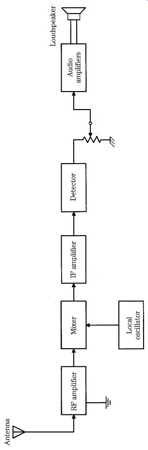
FIG. 1 Block diagram of a single-conversion superheterodyne receiver.
The main attribute of the superheterodyne receiver is that it converts the radio signal's RF frequency to a standard frequency for further processing. Although today the new frequency, called the intermediate frequency (IF), might be either higher or lower than the RF frequencies, early superheterodyne receivers were always down-converted to a lower IF frequency (IF _ RF). The reason was purely practical; in those days, higher frequencies were more difficult to process than lower frequencies. Even today, because variable tuned circuits still tend to offer different performance over the band being tuned, converting to a single IF frequency and obtaining most of the gain and selectivity functions at the IF allows more uniform over all performance over the entire range being tuned.
A superheterodyne receiver works by frequency converting ("heterodyning"- the "super" part is 1920s vintage advertising hype) the RF signal. This occurs by nonlinearly mixing the incoming RF signal with a local oscillator (LO) signal. When this process is done, disregarding noise, the output spectrum will contain a large variety of signals according to:

(Eqn. 1)
...where...
FRF is the frequency of the RF signal FLO is the frequency of the local oscillator m and n are either zero or integers (0, 1, 2, 3 . . . . n).
Equation (Eqn. 1) means that there will be a large number of signals at the output of the mixer, although for the most part the only ones that are of immediate concern to understanding basic superheterodyne operation are those for which m and n are either 0 or 1. Thus, for our present purpose, the output of the mixer will be the fundamentals (FRF and FLO) and the second-order products (FLO _ FRF and FLO _ FRF), as seen in Fig. 2. Some mixers, notably those described as double-balanced mixers (DBM), suppress FRF and FLO in the mixer output, so only the second-order sum and difference frequencies exist with any appreciable amplitude. This case is simplistic and is used only for this discussion. Later on, we will look at what happens when third-order (2F1 _ F2 and 2F2 _ F1) and fifth-order (3F1 _ 2F2 and 3F2 _ 2F1) be come large.
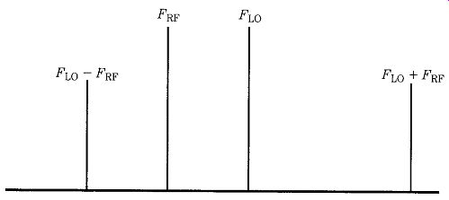
FIG. 2 Combining the LO and RF frequencies in a mixer product second-order
products of LO _ RF and LO _ RF.
Notice that the local oscillator frequency can be either higher than the RF frequency (high-side injection) or lower than the RF frequency (low-side injection).
There is ordinarily no practical reason to prefer one over the other, except that it will make a difference whether the main tuning dial reads high-to-low or low-to-high. The candidates for IF are the sum (LO _ RF) and difference (LO _ RF) second order products found at the output of the mixer. A high-Q tuned circuit following the mixer will select which of the two are used. Consider an example. Suppose a super het radio has an IF frequency of 455 kHz and the tuning range is 540 to 1700 kHz.
Because the IF is lower than any frequency within the tuning range, the difference frequency will be selected for the IF. The local oscillator is set to be high-side injection, so it will tune from 540 _ 455 _ 995 kHz to 1700 _ 455 _ 2155 kHz.
Front-end circuits
The principal task of the "front-end" section of the receiver in Fig. 1 is to per form the frequency conversion. But in many radio receivers, there are additional functions. In some cases (but not all), an RF amplifier will be used ahead of the mixer. Typically, these amplifiers have a gain of 3 to 10 dB, with 5 to 6 dB being very common. The tuning for the RF amplifier is sometimes a broad bandpass fixed frequency filter that admits an entire band. In other cases, it is a narrow band, but vari able frequency, tuned circuit.
Intermediate frequency (IF) amplifier The IF amplifier is responsible for providing most of the gain in the receiver as well as the narrowest bandpass filtering. It is a high-gain, usually multistaged, single frequency tuned radio-frequency amplifier. For example, one receiver block diagram lists 120 dB of gain from antenna terminals to audio output, of which 85 dB are pro vided in the 8.83-MHz IF amplifier chain. In the example of Fig. 1, the receiver is a single-conversion design, so there is only one IF amplifier section.
Detector
The detector demodulates the RF signal and recovers whatever audio (or other information) is to be heard by the listener. In a straight AM receiver, the detector will be an ordinary half-wave rectifier and ripple filter and is called an envelope detector.
In other detectors, notably double-sideband suppressed carrier (DSBSC), single sideband suppressed carrier (SSBSC or SSB), or continuous wave (CW or Morse telegraphy), a second local oscillator, usually called a beat frequency oscillator (BFO), operating near the IF frequency, is heterodyned with the IF signal. The resultant difference signal is the recovered audio. That type of detector is called a product detector. Many AM receivers today have a sophisticated synchronous detector rather than the simple envelope detector.
Audio amplifiers
The audio amplifiers are used to finish the signal processing. They also boost the output of the detector to a usable level to drive a loudspeaker or set of earphones.
The audio amplifiers are sometimes used to provide additional filtering. It is quite common to find narrowband filters to restrict audio bandwidth or notch filters to eliminate interfering signals that make it through the IF amplifiers intact.
Three basic areas of receiver performance must be considered. Although inter related, they are sufficiently different to merit individual consideration: noise, static, and dynamic. We will look at all of these areas, but first let's look at the units of mea sure that we will use in this series.
Units of measure
Input signal voltage
Input signal levels, when specified as a voltage, are typically stated in either microvolts (_V) or nano-volts (nV); the volt is simply too large a unit for practical use on radio receivers. Signal input voltage (or sometimes power level) is often used as part of the sensitivity specification or as a test condition for measuring certain other performance parameters.
Two forms of signal voltage that are used for input voltage specification: source voltage (VEMF) and potential difference (VPD), as illustrated in Fig. 3 (after Dyer, 1993). The source voltage (VEMF) is the open terminal (no load) voltage of the signal generator or source while the potential difference (VPD) is the voltage that appears across the receiver antenna terminals with the load connected (the load is the receiver antenna input impedance, Rin). When Rs = Rin, the preferred "matched impedances" case in radio receiver systems, the value of VPD is one-half VEMF. This can be seen in Fig. 3 by noting that Rs and Rin form a voltage divider network driven by VEMF and with VPD as the output.
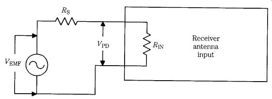
FIG. 3 Equivalent circuit of a receiver input network.
dBm
This unit refers to decibels relative to 1 mW dissipated in a 50-ohm resistive impedance (defined as the 0-dBm reference level) and is calculated from 10 log (PW/0.001) or 10 log (PMW). In the noise voltage case, 0.028 _V in 50-ohm , the power is V2/50, or 5.6 _ 10_10 W, which is 5.6 _ 10_7 mW. In dBm notation, this value is 10 log (5.6 _ 10_7), or _62.5 dBm.
dBmV
This unit is used in television receiver systems in which the system impedance is 75 ohm rather than the 50-ohm normally used in other RF systems. It refers to the signal voltage, measured in decibels, with respect to a signal level of 1 millivolt (1 mV) across a 75 ohm resistance (0 dBmv). In many TV specs, 1 mV is the full quieting signal that produces no "snow" (i.e., noise) in the displayed picture.
dB_V
This unit refers to a signal voltage, measured in decibels, relative to 1 _V developed across a 50-ohm resistive impedance (0 dB_V). For the case of our noise signal voltage, the level is 0.028 _V, which is the same as _31.1 dB_V. The voltage used for this measurement is usually the VEMF, so to find VPD, divide it by two after converting dB_V to _V. To convert dB_V to dBm, merely subtract 113; i.e., 100 dB_V _ _13 dBm.
It requires only a little algebra to convert signal levels from one unit of measure to another. This job is sometimes necessary when a receiver manufacturer mixes methods in the same specifications sheet. In the case of dBm and dB_V, 0 dB_V is 1 _V VEMF, or a VPD of 0.5 _V, applied across 50-ohm , so the power dissipated is 5 _ 10_15 watts, or _113 dBm. To convert from dB_V to dBm add 107 dB to the dBm figure.
Noise A radio receiver must detect signals in the presence of noise. The signal-to-noise ratio (SNR) is the key here because a signal must be above the noise level before it can be successfully detected and used.
Noise comes in a number of different guises, but for sake of this discussion, you can divide them into two classes1: sources external to the receiver and sources internal to the receiver. You can do little about the external noise sources, for they consist of natural and human-made electromagnetic signals that fall within the pass band of the receiver. Figure 4 shows an approximation of the external noise situation from the middle of the AM broadcast band to the low end of the VHF region. You must select a receiver that can cope with external noise sources-especially if the noise sources are strong.
Some natural external noise sources are extraterrestrial. For example, if you aim a beam antenna at the eastern horizon prior to sunrise, a distinct rise of noise level occurs as the Sun slips above the horizon-especially in the VHF region. The reverse occurs in the west at sunset, but is less dramatic, probably because atmospheric ionization decays much slower than it is generated. During World War II, it is reported that British radar operators noted an increase in received noise level any time the Milky Way was above the horizon, decreasing the range at which they could detect in-bound bombers. There is also some well-known, easily observed noise from the planet Jupiter in the 18- to 30-MHz band (Carr, 1994 and 1995).
[1. It is said that people are divided into two classes: those who divide everything into two classes and those who don't.]
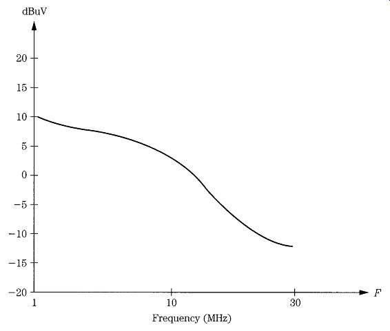
FIG. 4 External noise from about 1 to 140 MHz.
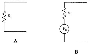
FIG. 5 (A) Ideal resistor and (B) resistor with noise thermal source.
The receiver's internal noise sources are affected by the design of the receiver.
Ideal receivers produce no noise of their own, so the output signal from the ideal receiver would contain only the noise that was present at the input along with the radio signal. But real receiver circuits produce a certain level of internal noise of their own. Even a simple fixed-value resistor is noisy. Figure 5A shows the equivalent circuit for an ideal, noise-free resistor. Figure 5B shows a practical real-world resistor. The noise in the real-world resistor is represented in Fig. 5B by a noise volt age source, Vn, in series with the ideal, noise-free resistance, Ri. At any temperature above Absolute Zero (0 K or about _273 C) electrons in any material are in constant random motion. Because of the inherent randomness of that motion, however, there is no detectable current in any one direction. In other words, electron drift in any single direction is canceled over even short time periods by equal drift in the opposite direction. Electron motions are therefore statistically decorrelated. There is, however, a continuous series of random current pulses generated in the material, and those pulses are seen by the outside world as noise signals.
If a shielded 50-ohm resistor is connected across the antenna input terminals of a radio receiver (Fig. 6), the noise level at the receiver output will increase by a predictable amount over the short-circuit noise level. Noise signals of this type are called by several names: thermal agitation noise, thermal noise, or Johnson noise. This type of noise is also called white noise because it has a very broadband (nearly gaussian) spectral density. The thermal noise spectrum is dominated by mid frequencies and is essentially flat. The term white noise is a metaphor developed from white light, which is composed of all visible color frequencies. The expression for such noise is:
(Eqn. 2)
where.....
Vn is the noise potential in volts (V) K is Boltzmann's constant (1.38 x 10^-23 J/ K) T is the temperature in degrees Kelvin ( K), normally set to 290 or 300 K by convention.
R is the resistance in ohms (_)
B is the bandwidth in hertz (Hz).
Vn _ 24 KTBR
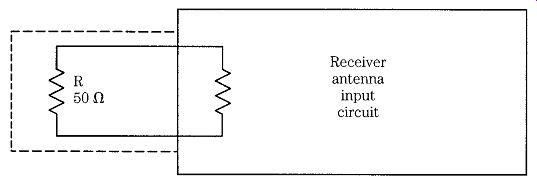
FIG. 6 Noise test set-up for demonstration purposes only.
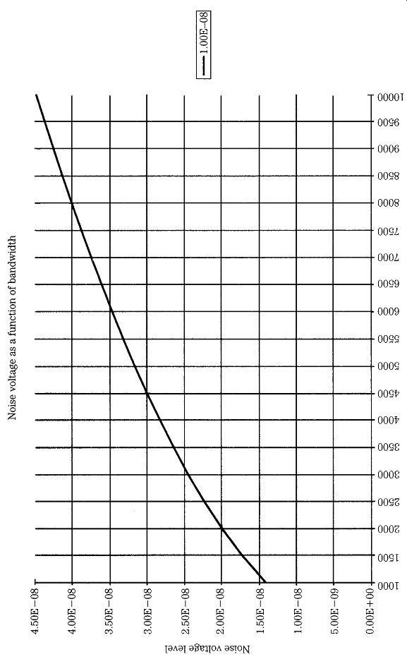
FIG. 7 Thermal noise in bandwidths of 100 Hz to 10 kHz.
Table 1. Noise levels tabulated for three bandwidths commonly found in receivers
Example:
Find the noise voltage in a circuit containing only a 50-ohm resistor if the band width is 1000 Hz.
Table 1 and Fig. 7 show noise values for a 50-ohm resistor at various band widths out to 5 and 10 kHz, respectively.
Because different bandwidths are used for different reception modes, it is common practice to delete the bandwidth factor in Eq. (Eqn. 2) and write it in the form:

(Eqn. 3)
With Eq. (Eqn. 3), you can find the noise voltage for any particular bandwidth by taking its square root and multiplying it by the equation. This equation is essentially the solution of the previous equation normalized for a 1-Hz bandwidth.
Signal-to-noise ratio (SNR or Sn) Receivers can be evaluated on the basis of signal-to-noise ratio (S/N or "SNR"), sometimes denoted Sn. The goal of the designer is to enhance the SNR as much as possible. Ultimately, the minimum signal level detectable at the output of an amplifier or radio receiver is that level which appears just above the noise floor level. There fore, the lower the system noise floor, the smaller the minimum allowable signal.
Noise factor, noise figure, and noise temperature
The noise performance of a receiver or amplifier can be defined in three different, but related, ways: noise factor (Fn), noise figure (NF), and equivalent noise temperature (Te); these properties are definable as a simple ratio, decibel ratio, or Kelvin temperature, respectively.
Noise factor (Fn)
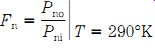
For components such as resistors, the noise factor is the ratio of the noise produced by a real resistor to the simple thermal noise of an ideal resistor. The noise factor of a radio receiver (or any system) is the ratio of output noise power (Pno) to input noise power (Pni):
(Eqn. 4)
In order to make comparisons easier, the noise factor is usually measured at the standard temperature (To) of 290 K (standardized room temperature); although in some countries 299 K or 300 K are commonly used (the differences are negligible).
It is also possible to define noise factor Fn in terms of output and input S/N ratio:

(Eqn. 5) ...where...
Sni is the input signal-to-noise ratio Sno is the output signal-to-noise ratio.
Noise figure (NF) The noise figure is a frequently used measure of a receiver's "goodness," or its departure from "idealness." Thus, it is a figure of merit. The noise figure is the noise factor converted to decibel notation:
NF = 10 log (Fn), (Eqn. 6) where
NF = the noise figure in decibels (dB)
Fn = the noise factor
log refers to the system of base-10 logarithms.
Noise temperature (Te)--The noise "temperature" is a means for specifying noise in terms of an equivalent temperature. Evaluating the noise equations shows that the noise power is directly proportional to temperature in degrees Kelvin and also that noise power collapses to zero at the temperature of Absolute Zero (0 K).
Notice that equivalent noise temperature Te is not the physical temperature of the amplifier but rather a theoretical construct that is an equivalent temperature that produces that amount of noise power. The noise temperature is related to the noise factor by:

(Eqn. 7) and to noise figure by:

(Eqn. 8)
Noise temperature is often specified for receivers and amplifiers in combination with, or in lieu of the noise figure.
Noise in cascade amplifiers
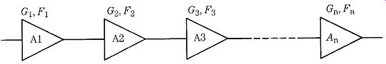
FIG. 8 Cascade amplifier chain.
A noise signal is seen by any following amplifier as a valid input signal. Each stage in the cascade chain (Fig. 8) amplifies both signals and noise from previous stages and also contributes some additional noise of its own. Thus, in a cascade amplifier, the final stage sees an input signal that consists of the original signal and noise amplified by each successive stage plus the noise contributed by earlier stages.
The overall noise factor for a cascade amplifier can be calculated from Friis' noise equation:
(Eqn. 9) where...
Fn is the overall noise factor of N stages in cascade
F1 is the noise factor of stage 1
F2 is the noise factor of stage 2
Fn is the noise factor of the nth stage
G1 is the gain of stage 1
G2 is the gain of stage 2
Gn-1 is the gain of stage (n - 1).
As you can see from Friis' equation, the noise factor of the entire cascade chain is dominated by the noise contribution of the first stage or two. High-gain, low-noise amplifiers typically use a low-noise amplifier circuit for only the first stage or two in the cascade chain. Thus, you will find a LNA at the feedpoint of a satellite receiver's dish antenna, and possibly another one at the input of the receiver module itself, but other amplifiers in the chain are more modest.
The matter of signal-to-noise ratio (S/N) is sometimes treated in different ways that each attempt to crank some reality into the process. The signal-plus-noise to-noise ratio (S + N/N) is found quite often. As the ratios get higher, the S/N and S + N/N converge (only about 0.5-dB difference at ratios as little as 10 dB). Still another variant is the SINAD (signal-plus-noise-plus-distortion-to-noise) ratio. The SINAD measurement takes into account most of the factors that can deteriorate reception.
Receiver noise floor
The noise floor of the receiver is a statement of the amount of noise produced by the receiver's internal circuitry and directly affects the sensitivity. The noise floor is typically expressed in dBm. The noise floor specification is evaluated as follows: the more negative the better. The best receivers have noise floor numbers of less than -130 dBm, and some very good receivers offer numbers of -115 dBm to -130 dBm.
The noise floor is directly dependent on the bandwidth used to make the measurement. Receiver advertisements usually specify the bandwidth, but be careful to note whether the bandwidth that produced the very good performance numbers is also the bandwidth that you'll need for the mode of transmission you want to receive. If, for example, you are interested only in weak 6-kHz wide AM signals and the noise floor is specified for a 250-Hz CW filter then the noise floor might be too high for your use.
Static measures of performance
The two principal static levels of performance for radio receivers are sensitivity and selectivity. The sensitivity refers to the level of input signal required to produce a usable output signal (variously defined). The selectivity refers to the ability of the receiver to reject adjacent channel signals (again, variously defined). Look at both of these factors. Remember, however, that in modern, high-performance radio receivers the static measures of performance might also be the least relevant com pared with the dynamic measures.
Sensitivity
Sensitivity is a measure of the receiver's ability to pick up ("detect") signals and is usually specified in microvolts (uV). A typical specification might be "0.5-uV sensitivity." The question to ask is "relative to what?" The sensitivity number in microvolts is meaningless unless the test conditions are specified. For most commercial receivers, the usual test condition is the sensitivity required to produce a 10-dB signal-plus-noise-to-noise (S + N/N) ratio in the mode of interest. For example, if only one sensitivity figure is given, one must find out what bandwidth is being used: 5 to 6 kHz for AM, 2.6 to 3 kHz for single sideband, 1.8 kHz for radio teletype, or 200 to 500 Hz for CW.
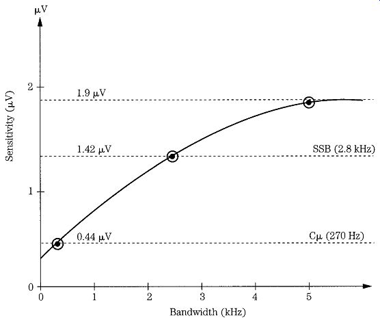
FIG. 9 Comparison of signal levels required for 10-dB SNR for 270-Hz and 2.8
and 5-kHz bandwidths.
Bandwidth affects sensitivity measurements. Indeed, one place where "creative spec writing" takes place for commercial receivers is that the advertisements will cite the sensitivity for a narrow-bandwidth mode (e.g., CW), and the other specifications are cited for a more commonly used wider bandwidth mode (e.g., SSB). In one particularly egregious example, an advert claimed a sensitivity number that was applicable to the CW mode bandwidth only, yet the 270-Hz CW filter was an expensive option that had to be specially ordered separately! The amount of sensitivity improvement is seen by some simple numbers. Recall that a claim of "X _V" sensitivity refers to some standard such as "X _V to produce a 10-dB signal-to-noise ratio." Consider the case where the main mode for a high frequency (HF) shortwave receiver is AM (for international broadcasting), and the sensitivity is 1.9 _V for 10 dB SNR, and the bandwidth is 5 kHz. If the bandwidth were reduced to 2.8 kHz for SSB then the sensitivity improves by the square root of the ratio, or /2.8. If the bandwidth is further reduced to 270 Hz (i.e., 0.27 kHz) for CW then the sensitivity for 10 dB SNR is /0.27. The 1.9-_V AM sensitivity therefore translates to 1.42 _V for SSB and 0.44 _V for CW. If only the CW version is given then the receiver might be made to look a whole lot better, even though the typical user might never use the CW mode (note differences in Fig. 9).
The sensitivity differences also explain why weak SSB signals can be heard under conditions when AM signals of similar strength have disappeared into the noise or why the CW mode has as much as 20-dB advantage over SSB, ceterus paribus.
In some receivers, the difference in mode (AM, SSB, RTTY, CW, etc.) can conceivably result in sensitivity differences that are more than the differences in the bandwidths associated with the various modes. The reason is that there is some times a "processing gain" associated with the type of detector circuit used to de modulate the signal at the output of the IF amplifier. A simple AM envelope detector is lossy because it consists of a simple diode (1N60, etc.) and an RC filter (a passive circuit). Other detectors (product detector for SSB and synchronous AM detectors) have their own signal gain, so they might produce better sensitivity numbers than the bandwidth suggests.
Another indication of sensitivity is minimum detectable signal (MDS) and is usually specified in dBm. This signal level is the signal power at the antenna input terminal of the receiver required to produce some standard S + N/N ratio, such as 3 or 10 dB (Fig. 10). In radar receivers, the MDS is usually described in terms of a single pulse return and a specified S+N/N ratio. Also, in radar receivers, the sensitivity can be improved by integrating multiple pulses. If N return pulses are integrated, then the sensitivity is improved by a factor of N if coherent detection is used, and if noncoherent detection is used.
Modulated signals represent a special case. For those sensitivities, it is common to specify the conditions under which the measurement is made. For example, in AM receivers, the sensitivity to achieve 10-dB SNR is measured with the input signal modulated 30% by a 400- or 1000-Hz sinusoidal tone.
An alternate method is sometimes used for AM sensitivity measurements- especially in servicing consumer radio receivers (where SNR might be a little hard to measure with the equipment normally available to technicians who work on those radios). This is the "standard output conditions" method. Some manuals specify the audio signal power or audio signal voltage at some critical point, when the 30% modulated RF carrier is present. In one automobile radio receiver, the sensitivity was specified as "X _V to produce 400 mW across 8-ohm resistive load substituted for the loudspeaker when the signal generator is modulated 30% with a 400-Hz audio tone." The cryptic note on the schematic showed an output sine wave across the loud speaker with the label "400 mW in 8 _ (1.79 volts), @30% mod. 400 Hz, 1 _V RF." The sensitivity is sometimes measured essentially the same way, but the signal levels will specify the voltage level that will appear at the top of the volume control, or out put of the detector/filter, when the standard signal is applied. Thus, there are two ways seen for specifying AM sensitivity: 10 dB SNR and standard output conditions.
There are also two ways to specify FM receiver sensitivity. The first is the 10-dB SNR method (i.e., the number of microvolts of signal at the input terminals required to produce a 10-dB SNR when the carrier is modulated by a standard amount). The measure of FM modulation is deviation expressed in kilohertz. Sometimes, the full deviation for that class of receiver is used and for others a value that is 25 to 35% of full deviation is specified.
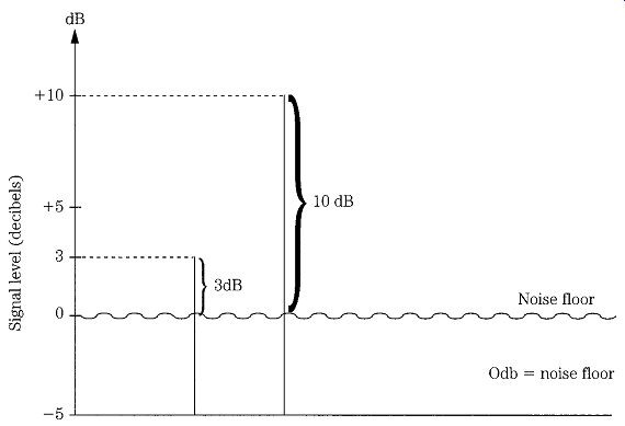
FIG. 10 Minimum detectable signal (MDS) defined for two different standards
(3-dB SNR and 10-dB SNR).
The second way to measure FM sensitivity is the level of signal required to re duce the no-signal noise level by 20 dB. This is the "20-dB quieting sensitivity of the receiver." If you tune between signals on a FM receiver, you will hear a loud "hiss" signal. Some of that noise is externally generated, while some is internally generated.
When a FM signal appears in the passband, that hiss is suppressed-even if the FM carrier is unmodulated. The quieting sensitivity of a FM receiver is a statement of the number of microvolts required to produce some standard quieting level, usually 20 dB.
Pulse receivers, such as radar and pulse communications units, often use the tangential sensitivity as the measure of performance, which is the amplitude of pulse signal required to raise the noise level by its own RMS amplitude (Fig. 11).
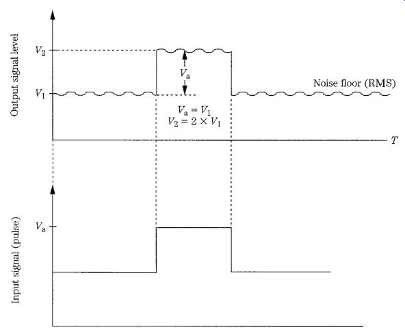
FIG. 11 Tangential sensitivity measurement.
Selectivity
Although no receiver specification is unimportant, if one had to choose between sensitivity and selectivity, the proper choice most of the time would be to take selectivity.
Selectivity is the measure of a receiver's ability to reject adjacent channel interference. Or put another way, it's the ability to reject interference from signals on frequencies close to the desired signal frequency.
To understand selectivity requirements, you must first understand a little bit of the nature of real radio signals. An unmodulated radio carrier theoretically has an infinitesimal (near-zero) bandwidth (although all real unmodulated carriers have a very narrow, but nonzero, bandwidth because they are modulated by noise and other artifacts). As soon as the radio signal is modulated to carry information, however, the bandwidth spreads.
An on/off telegraphy (CW) signal spreads out either side of the carrier frequency an amount that depends on the sending speed and the shape of the keying waveform.
Figure 12 compares two radio-teletype signals with 200 Hz (Fig. 12A) and 800 Hz (Fig. 12B) mark/space separation. Notice how the sidebands spread out from the main mark and space signals.
An AM signal spreads out an amount equal to twice the highest audio modulating frequencies. For example, a communications AM transmitter will have audio components from 300 to 3000 Hz, so the AM waveform will occupy a spectrum that is equal to the carrier frequency (F) plus/minus the audio bandwidth (F _ 3000 Hz in the case cited).
FIG. 12 (A) Spectrum for 200-Hz RTTY and (B) spectrum for 800-Hz RTTY.
FIG. 12 Continued.
An FM carrier spreads out according to the deviation. For example, a narrow band FM land mobile transmitter with 5-kHz deviation spreads out _5 kHz and FM broadcast transmitters spread out _75 kHz.
An implication of the radio signal bandwidth is that the receiver must have sufficient bandwidth to recover all of the signal. Otherwise, information might be lost and the output is distorted. On the other hand, allowing too much bandwidth in creases the noise picked up by the receiver and thereby deteriorates the SNR. The goal of the selectivity system of the receiver is to match the bandwidth of the receiver to that of the signal. That is why receivers will use a bandwidth of 270 or 500 Hz for CW, 2 to 3 kHz for SSB, and 4 to 6 kHz for AM signals. They allow you to match the receiver bandwidth to the transmission type.
The selectivity of a receiver has a number of aspects that must be considered: front-end bandwidth, IF bandwidth, IF shape factor, and the ultimate (distant frequency) rejection.
Front-end bandwidth
The "front end" of a modern superheterodyne radio receiver is the circuitry be tween the antenna input terminal and the output of the first mixer stage. Front-end selectivity is important because it keeps out-of-band signals from afflicting the receiver. For example, AM broadcast band transmitters located nearby can easily over load a poorly designed shortwave receiver. Even if these signals are not heard by the operator (as they often are), they can desensitize a receiver or create harmonics and intermodulation products that show up as "birdies" or other types of interference on the receiver. Strong local signals can take a lot of the receiver's dynamic range and thereby make it harder to hear weak signals.
In some "crystal video" microwave receivers, that front end might be wide open without any selectivity at all, but in nearly all other receivers, some form of frequency selection will be present.
Two forms of frequency selection are typically found. A designer might choose to use only one of them in a design. Alternatively, both might be used in the design, but separately (operator selection). Or finally, both might be used together. These forms can be called the resonant frequency filter (Fig. 13A) and bandpass filter (Fig. 13B) approaches.
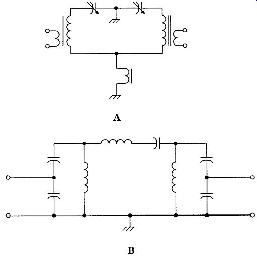
FIG. 13 (A) Resonant filter and (B) bandpass filter.
The resonant frequency approach uses LC elements tuned to the desired frequency to select which RF signals reach the mixer. In some receivers, these LC elements are designed to track with the local oscillator that sets the operating frequency. That's why you see two- section variable capacitors for AM broadcast receivers with two different capacitance ranges for the two sections; one section tunes the LO and the other section tunes the tracking RF input. In other designs, a separate tuning knob ("preselector" or "antenna") is used.
The other approach uses a sub-octave bandpass filter to admit only a portion of the RF spectrum into the front end. For example, a shortwave receiver that is de signed to take the HF spectrum in 1-MHz pieces might have an array of RF input bandpass filters that are each 1 MHz wide (e.g., 9 to 10 MHz).
In addition to these reasons, front-end selectivity also helps improve a receiver's image rejection and 1st IF rejection capabilities.
Image rejection
An image in a superheterodyne receiver is a signal that appears at twice the IF distant from the desired RF signal and is located on the opposite side of the LO frequency from the desired RF signal. In Fig. 14, a superheterodyne operates with a 455 kHz (i.e., 0.455 MHz) IF and is turned to 24.0 MHz (FRF). Because this receiver uses low-side LO injection, the LO frequency FLO is 24.0-0.455, or 23.545 MHz. If a signal appears at twice the IF below the RF (i.e., 910 kHz below FRF) and reaches the mixer then it too has a difference frequency of 455 kHz so it will pass right through the IF filtering as a valid signal. The image rejection specification tells how well this image frequency is suppressed. Normally, anything over about 70 dB is considered good.
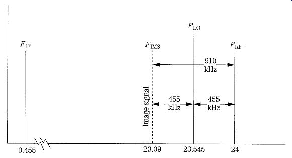
FIG. 14 The image response problem.
Tactics to reduce image response vary with the design of the receiver. The best approach, at design time, is to select an IF frequency that is high enough that the image frequency will fall outside the passband of the receiver front end. Some modern HF receivers use an IF of 8.83, 9, or 10.7 MHz or something similar. For image rejection, these frequencies are considerably better than 455-kHz receivers in the higher HF bands. However, a common trend is to double conversion. In most such designs, the first IF frequency is considerably higher than the RF, being in the range 35 to 60 MHz (50 MHz is common). This high IF makes it possible to suppress the VHF images with a simple low-pass filter. If the 24.0-MHz signal (above) were first up converted to 50 MHz (74-MHz LO), for example, the image would be at 124 MHz. The second conversion brings the IF down to one of the frequencies mentioned, or even 455 kHz. The lower frequencies are preferable to 50 MHz for bandwidth selectivity reasons because good-quality crystal, ceramic, or mechanical filters in those ranges filters are easily available.
First IF rejection
The first IF rejection specification refers to how well a receiver rejects radio signals operating on the receiver's first IF frequency. For example, if your receiver has a first IF of 8.83 MHz, it must be able to reject radio signals operating on that frequency when the receiver is tuned to a different frequency. Although the shielding of the receiver is also an issue with respect to this performance, the front-end selectivity affects how well the receiver performs against first IF signals. If there is no front-end selectivity to discriminate against signals at the IF frequency, then they arrive at the input of the mixer unimpeded. Depending on the design of the mixer, they then pass directly through to the high gain IF amplifiers and be heard in the receiver output.
IF bandwidth
Most of the selectivity of the receiver is provided by the filtering in the IF amplifier section. The filtering might be LC filters (especially if the principal IF is a low frequency, such as 50 kHz), a ceramic resonator, a crystal filter, or a mechanical filter. Of these, the mechanical filter is usually regarded as best, with the crystal filter and ceramic filters coming in next.
The IF bandwidth is expressed in kilohertz and is measured from the points on the IF frequency response curve where gain drops off _3 dB from the mid-band value (Fig. 15). This is why you will sometimes see selectivity referred to in terms such as "6 kHz between -3 dB points."
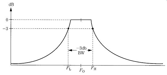
FIG. 15 IF bandwidth selectivity.
The IF bandwidth must be matched to the bandwidth of the received signal for best performance. If a too-wide bandwidth is selected then the received signal will be noisy and SNR deteriorates. If it is too narrow then you might experience difficulties recovering all of the information that was transmitted. For example, an AM broadcast band radio signal has audio components to 5 kHz, so the signal occupies up to 10 kHz of spectrum space (F +- 5 kHz). If a 2.8-kHz SSB IF filter is selected it will tend to sound "mushy" and distorted.
IF passband shape factor
The shape factor is a measure of the steepness of the receiver's IF passband and is taken by measuring the ratio of the bandwidth at -6 dB to the bandwidth at -60 dB. The general rule is that the closer these numbers are to each other, the better the receiver. Anything in the 1:1.5 to 1:1.9 region can be considered high quality, and anything worse than 1:3 is not worth looking at for "serious" receiver uses. If the numbers are between 1:1.9 and 1:3 then the receiver could be regarded as being middling but useful.
The importance of shape factor is that it modifies the bandwidth. The cited bandwidth (e.g., 2.8 kHz for SSB) does not take into account the effects of strong signals that are just beyond those limits. Such signals can easily "punch through" the IF selectivity if the IF passband "skirts" are not steep. After all, the steeper they are, the closer a strong signal can be without messing up the receiver's operation. Thus, selecting a receiver with a shape factor as close to the 1:1 ideal as possible (it's not, by the way) will result in a more usable radio.
Distant frequency ("ultimate") rejection
This specification tells something about the receiver's ability to reject very strong signals that are located well outside the receiver's IF passband. This number is stated in negative decibels, and the higher the number the better. An excellent receiver will have values in the -60- to -90-dB range, a middling receiver will see numbers in the -45- to-60-dB range, and a terrible receiver will be -44 or worse.
Stability
The stability specification measures how much the receiver frequency drifts as time elapses or temperature changes. The LO drift sets the overall stability of the receiver. This specification is usually given in terms of short-term drift and long-term drift (e.g., from crystal aging). The short-term drift is important in daily operation, and the long-term drift ultimately affects general dial calibration.
If the receiver is VFO controlled, or uses partial frequency synthesis (which combines VFO with crystal oscillators), then the stability is dominated by the VFO stability. In fully synthesized receivers, the stability is governed by the master reference crystal oscillator. If either an oven-controlled crystal oscillator (OCXO) or a temperature-compensated crystal oscillator (TCXO) is used for the master reference then stability on the order of 1 part in 108/ C is achievable.
For most users, the short-term stability is what is most important-especially when tuning SSB, ECSS, or RTTY signals. A common spec for a good receiver will be 50 Hz/h after a 3-h warm-up or 100 Hz/h after a 15-min warm-up. The smaller the drift the better the receiver.
The foundation of good stability is at design time. The local oscillator, or VFO portion of a synthesizer, must be operated in a cool, temperature-stable location within the equipment and must have the correct type of components. Capacitor temperature coefficients are often selected in order to cancel out temperature-related drift in inductance values.
Post-design time changes can also help, but these are less likely to be possible today than in the past. The chief cause of drift problems is heat. In the days of tube oscillators, the heat of the tubes produced lots of heat, which created drift. One popular receiver of the 1950s was an excellent performer, except for the drift of the VFO/LO. A popular modification was to insert metal panels backed with insulating material between the heat source (an IF amplifier chain) and the VFO case. Rather dramatic improvement resulted. In most modern solid-state receivers, however, space is not so easily found for such modifications.
One phenomenon seen on low-cost receivers and homebrew receivers of doubtful merit is mechanical frequency shifts. Although not seen on most modern receivers (even some very cheap designs), it was once a serious problem on less costly models. This problem is usually seen on VFO-controlled receivers in which vibration to the receiver cabinet imparts movement to either the inductor (L) or capacitor (C) element in a LC VFO. Mechanically stabilizing these components will work wonders.
AGC range and threshold
Modern communications receivers must be able to handle signals over the range of about 1,000,000:1. Tuning across a band occupied by signals of wildly varying strengths is hard on the ears and hard on the receiver's performance. As a result, most modern receivers have an automatic gain control (AGC) circuit that smooths out these changes. The AGC will reduce gain for strong signals and increase it for weak signals (AGC can be turned off on most HF communications receivers). The AGC range is the change of input signal (in dBuV) from some reference level (e.g., 1 uVEMF) to the input level that produces a 2-dB change in output level. Ranges of 90 to 110 dB are common.
The AGC threshold is the signal level at which the AGC begins to operate. If it is set too low, the receiver gain will respond to noise and irritate the user. If set too high, then the user will experience irritating shifts of output level as the band is tuned. AGC thresholds of 0.7 to 2.5 uV are common on decent receivers, with the better receivers being in the 0.7- to 1-uV range.
Another AGC specification sometimes seen deals with the speed of the AGC. Although sometimes specified in milliseconds, it is also frequently specified in subjective terms like "fast" and "slow." This specification refers to how fast the AGC responds to changes in signal strength. If set too fast, then rapidly keyed signals (e.g., CW) or noise transients will cause unnerving large shifts in receiver gain. If set too slow, then the receiver might as well not have an AGC. Many receivers provide two or more selections in order to accommodate different types of signals.
Now, let's examine what some authorities believe are the most important specifications for receivers used on crowded bands or in high electromagnetic interference (EMI) environments: the dynamic measures of performance. These include intermodulation distortion, 1-dB compression point, third-order intercept point, and blocking.
Dynamic performance
The dynamic performance specifications of a radio receiver are those that deal with how the receiver performs in the presence of very strong signals-either co-channel or adjacent channel. Until about the 1960s, dynamic performance was somewhat less important than static performance for most users. However, today the role of dynamic performance is probably more critical than static performance because of crowded band conditions.
There are at least two reasons for this change in outlook (Dyer, 1993). First, in the 1960s, receiver designs evolved from tubes to solid state. The new solid-state amplifiers were somewhat easier to drive into nonlinearity than tube designs. Second, there has been a tremendous increase in radio-frequency signals on the air.
There are far more transmitting stations than ever before, and there are far more sources of electromagnetic interference (EMI, the pollution of the air waves) than in prior decades. With the advent of new and expanded wireless services available to an ever widening market, the situation can only worsen. For this reason, it is now necessary to pay more attention to the dynamic performance of receivers than in the past.
Intermodulation products Understanding the dynamic performance of the receiver requires knowledge of intermodulation products (IP) and how they affect receiver operation. Whenever two signals are mixed together in a nonlinear circuit, a number of products are created according to mF1 _ nF2, where m and n are either integers or zero. Mixing can occur in either the mixer stage of a receiver front end or in the RF amplifier (or any outboard preamplifiers used ahead of the receiver) if the RF amplifier is overdriven by a strong signal.
It is also theoretically possible for corrosion on antenna connections, or even rusted antenna screw terminals to create IPs under certain circumstances. In some alleged cases, a rusty downspout on a house rain gutter caused reradiated mixed signals. However, all such cases that I've heard of have that distant third- or fourth party quality ("I know a guy whose best friend's brother-in-law saw . . .") that suggests a profound unconfirmability. I know of no first-hand accounts verified by a technically competent person.
The spurious IP signals are shown graphically in Fig. 16. Given input signal frequencies of F1 and F2, the main IPs are:
Second order: F1+- F2
Third order: 2F1 +- F2
2F2 +- F1
Fifth order: 3F1 +- 2F2
3F2 +- 2F1
…of these, the third-order difference signals (2F1 - F2 and 2F2 - F1) are the most serious because they typically fall close to the RF frequency.
When an amplifier or receiver is overdriven, the second-order content of the output signal increases as the square of the input signal level, and the third-order responses increase as the cube of the input signal level.
Consider the case where two HF signals, F1 = 10 MHz and F2 = 15 MHz, are mixed together. The second-order IPs are 5 and 25 MHz; the third-order IPs are 5, 20, 35, and 40 MHz; and the fifth-order IPs are 0, 25, 60, and 65 MHz. If any of these are inside the passband of the receiver then they can cause problems. One such problem is the emergence of "phantom" signals at the IP frequencies. This effect is often seen when two strong signals (F1 and F2) exist and can affect the front end of the receiver, and one of the IPs falls close to a desired signal frequency, Fd. If the receiver were tuned to 5 MHz, for example, a spurious signal would be found from the F1 - F2 pair.
Another example is seen from strong in-band, adjacent-channel signals. Consider a case where the receiver is tuned to a station at 9610 kHz, and there are also very strong signals at 9600 and 9605 kHz. The near (in-band) IP products are:
Third order:
9595 kHz (F = 15 kHz)
9610 kHz ( F = 0 kHz) [On channel!]
Fifth order:
9590 kHz ( F = 20 kHz)
9615 kHz ( F = 5 kHz).
Notice that one third-order product is on the same frequency as the desired signal and could easily cause interference if the amplitude is sufficiently high. Other third- and fifth-order products might be within the range where interference could occur, especially on receivers with wide bandwidths.
The IP orders are theoretically infinite because there are no bounds on either m or n. However, in practical terms, because each successively higher order IP is reduced in amplitude compared with its next lower order mate, only the second-order, third-order, and fifth-order products usually assume any importance. Indeed, only the third-order is normally used in receiver specifications sheets.
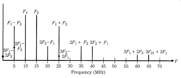
FIG. 16 Intermodulation products of second-order, third-order, and fifth-order.
-1-dB compression point
An amplifier produces an output signal that has a higher amplitude than the in put signal. The transfer function of the amplifier (indeed, any circuit with output and input) is the ratio OUT/IN, so for the power amplification of a receiver RF amplifier, it is Po /Pin (or, in terms of voltage, Vo /Vin). Any real amplifier will saturate, given a strong enough input signal (see Fig. 17). The dotted line represents the theoretical output level for all values of input signal (the slope of the line represents the gain of the amplifier). As the amplifier saturates (solid line), however, the actual gain begins to depart from the theoretical at some level of input signal (Pin1). The -1-dB compression point is that output level at which the actual gain departs from the theoretical gain by -1 dB.
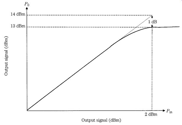
FIG. 17 1-dB compression point phenomenon.
The -1-dB compression point is important when considering either the RF amplifier ahead of the mixer (if any) or any outboard preamplifiers that are used. The -1-dB compression point is the point at which intermodulation products begin to emerge as a serious problem. Also, harmonics are generated when an amplifier goes into compression. A sine wave is a "pure" signal because it has no harmonics (all other waveshapes have a fundamental plus harmonic frequencies). When a sine wave is distorted, however, harmonics arise. The effect of the compression phenomenon is to distort the signal by clipping the peaks, thus raising the harmonics and intermodulation distortion products.
Third-order intercept point
It can be claimed that the third-order intercept point (TIP) is the single most important specification of a receiver's dynamic performance because it predicts the performance as regards intermodulation, cross-modulation, and blocking desensitization.
Third-order (and higher) intermodulation products (IP) are normally very weak and do not exceed the receiver noise floor when the receiver is operating in the linear region. But as input signal levels increase, forcing the front end of the receiver toward the saturated nonlinear region, the IP emerges from the noise (Fig. 18) and begins to cause problems. When this happens, new spurious signals appear on the band and self-generated interference begins to arise.
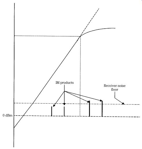
FIG. 18 As signal input levels rise, IP spurs emerge from the noise level.
Figure 19 shows a plot of the output signal vs the fundamental input signal.
Notice the output compression effect that was shown earlier in Fig. 17. The dotted gain line continuing above the saturation region shows the theoretical output that would be produced if the gain did not clip. It is the nature of third-order products in the output signal to emerge from the noise at a certain input level and increase as the cube of the input level. Thus, the slope of the third-order line increases 3 dB for every 1-dB increase in the response to the fundamental signal. Although the output response of the third-order line saturates similarly to that of the fundamental signal, the gain line can be continued to a point where it intersects the gain line of the fundamental signal. This point is the third-order intercept point (TOIP).
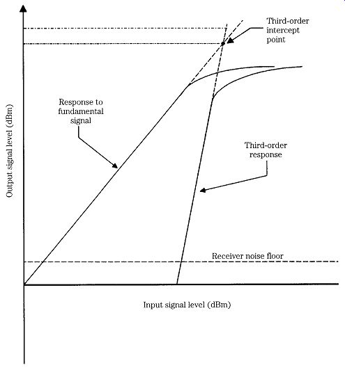
FIG. 19 Third-order intercept point (TOIP).
Interestingly enough, one receiver feature that can help reduce IP levels back down under the noise is the use of a front-end attenuator (a.k.a. input attenuator).
Even a few dB of input attenuation is often enough to drop the IPs back into the noise while afflicting the desired signals only a small amount.
Other effects that reduce the overload caused by a strong signal also help. I've seen situations in amateur radio operations where the apparent third-order performance of a receiver improved dramatically when a lower gain antenna was used. The late J. H. Thorne (K4NFU) demonstrated the effect to me on a VHF band using a spectrum analyzer/receiver. This instrument is a swept receiver that displays an out put on an oscilloscope screen that is amplitude vs frequency, so a single signal shows as a spike. A strong, local ham 2-m band repeater came on the air every few seconds, and you could observe the second- and third-order IPs along with the fundamental repeater signal. Other strong signals were also on the air, but just outside the 2-m ham band. Inserting a 6-dB barrel attenuator in the input ("antenna") line eliminated the IP products, showing just the actual signals. Rotating a directional antenna away from the direction of the interfering signal will also accomplish this effect in many cases.
Preamplifiers are popular receiver accessories, but can often reduce, rather than enhance, performance. Two problems commonly occur (assuming that the pre amp is a low-noise device; if not, then there are three). The best-known problem is that the preamp amplifies noise as much as signals, and although it makes the signal louder, it also makes the noise louder by the same amount. Because the signal-to noise ratio is important, you cannot improve the situation. Indeed, if the preamp is itself noisy, it will deteriorate the SNR. The other problem is less well-known, but potentially more devastating. If the increased signal levels applied to the receiver drive the receiver nonlinear, then IPs begin to emerge. Poole (1995) reported that another 2-m operator informed him that Poole's transmission was being heard at several spots on the band. Poole discovered that the other chap was using two preamps in cascade (!) to achieve more gain and that disconnecting them caused " Poole's spurs" to evaporate. That was clearly a case of a preamplifier messing up, rather than improving, a receiver's performance.
When evaluating receivers, a TOIP of +5 to +20 dBm is excellent performance, up to +27 dBm is relatively easily achievable, and +35 dBm has been achieved with good design; anything greater than +50 dBm is close to miraculous (but attainable). Receivers are still regarded as good performers in the 0- to +5-dBm range and as middling performers in the -10- to 0-dBm range. Anything below -10 dBm is a not too-wonderful machine to own. A general rule is to buy the best third-order intercept performance that you can afford-especially if strong signal sources are in your vicinity.
Dynamic range
The dynamic range of a radio receiver is the range from the minimum discernible signal to the maximum allowable signal (measured in decibels, dB). Although this simplistic definition is conceptually easy to understand, in the concrete it's a little more complex. Several definitions of dynamic range are used (Dyer, 1993).
One definition of dynamic range is that it is the input signal difference between the sensitivity figure (e.g., 0.5 uV for 10 dB S + N/N) and the level that drives the receiver far enough into saturation to create a certain amount of distortion in the output. This definition was common on consumer broadcast band receivers at one time (especially automobile radios, where dynamic range was somewhat more important because of mobility). A related definition takes the range as the distance in decibels from the sensitivity level and the -1-dB compression point. Still another definition, the blocking dynamic range, which is the range of signals from the sensitivity level to the blocking level (see below).
A problem with these definitions is that they represent single-signal cases so they do not address the receiver's dynamic characteristics. Dyer (1993) provides both a "loose" and a more formal definition that is somewhat more useful and is at least standardized. The loose version is that dynamic range is the range of signals over which dynamic effects (e.g., intermodulation, etc.) do not exceed the noise floor of the receiver. Dyer's recommendation for HF receivers is that the dynamic range is two-thirds of the difference between the noise floor and the third-order intercept point in a 3-kHz bandwidth. Dyer also states an alternative: dynamic range is the difference between the fundamental response input signal level and the third order intercept point along the noise floor, measured with a 3-kHz bandwidth. For practical reasons, this measurement is sometimes made not at the actual noise floor.
(which is sometimes hard to ascertain) but rather at 3 dB above the noise floor.
Magne and Sherwood (1987) provide a measurement procedure that produces similar results (the same method is used for many amateur radio magazine product reviews). Two equal-strength signals are input to the receiver at the same time. The frequency difference has traditionally been 20 kHz for HF and 30 to 50 kHz for VHF receivers (modern band crowding might indicate a need for a specification at 5-kHz separation on HF). The amplitudes of these signals are raised until the third-order distortion products are raised to the noise floor level.
For 20-kHz spacing, using the two-signal approach, anything over 90 dB is an excellent receiver, and anything over 80 dB is at least decent.
The difference between the single-to-signal and two-signal (dynamic) performance is not merely an academic exercise. Besides the fact that the same receiver can show as much as a 40-dB difference between the two measures (favoring the single-to-signal measurement), the most severe effects of poor dynamic range show up most in the dynamic performance.
Blocking
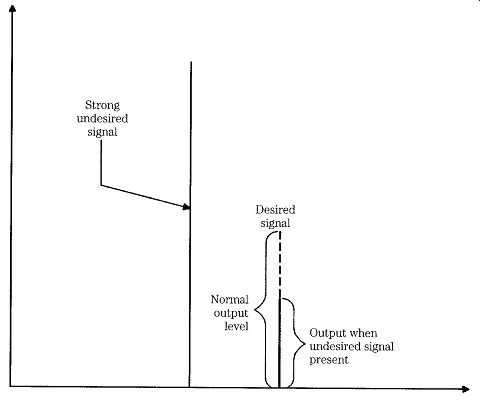
FIG. 20 The blocking, or "desensitization," phenomenon.
The blocking specification refers to the ability of the receiver to withstand very strong off-tune signals that are at least 20 kHz (Dyer, 1993) away from the desired signal, although some use 100-kHz separation (Magne and Sherwood, 1987). When very strong signals appear at the input terminals of a receiver, they can desensitize the receiver (i.e., reduce the apparent strength of desired signals over what they would be if the interfering signal were not present).
Figure 20 shows the blocking behavior. When a strong signal is present, it takes up more of the receiver's resources than normal, so there is not enough of the output power budget to accommodate the weaker desired signals. But if the strong undesired signal is turned off then the weaker signals receive a full measure of the unit's power budget.
The usual way to measure blocking behavior is to input two signals, a desired signal at 60 dB_V and another signal 20 (or 100) kHz away at a much stronger level.
The strong signal is increased to the point where blocking desensitization causes a 3-dB drop in the output level of the desired signal. A good receiver will show 90 dB_V, with many being considerably better. An interesting note about modern receivers is that the blocking performance is so good that it's often necessary to specify the input level difference (dB) that causes a 1-dB drop, rather than a 3-dB drop, of the desired signal's amplitude (Dyer, 1993).
The phenomenon of blocking leads to an effect that is often seen as paradoxical on first blush. Many receivers are equipped with front-end attenuators that permit fixed attenuations of 1, 3, 6, 12, or 20 dB (or some subset of same) to be inserted into the signal path ahead of the active stages. When a strong signal that is capable of causing desensitization is present, adding attenuation often increases the level of the desired signals in the output-even though overall gain is reduced. This occurs be cause the overall signal that the receiver front end is asked to handle is below the threshold where desensitization occurs.
Cross-modulation
Cross-modulation is an effect in which amplitude modulation (AM) from a strong undesired signal is transferred to a weaker desired signal. Testing is usually done (in HF receivers) with a 20-kHz spacing between the desired and undesired signals, a 3-kHz IF bandwidth on the receiver, and the desired signal set to 1000 _VEMF (_53 dBm). The undesired signal (20 kHz away) is amplitude-modulated to the 30% level. This undesired AM signal is increased in strength until an unwanted AM output 20 dB below the desired signal is produced.
A cross-modulation specification > 100 dB would be considered decent performance. This figure is often not given for modern HF receivers, but if the receiver has a good third-order intercept point then it is likely to also have good cross-modulation performance.
Cross-modulation is also said to occur naturally-especially in transpolar and North Atlantic radio paths, where the effects of the aurora are strong. According to one (possibly apocryphal) legend there was something called the "Radio Luxembourg Effect" discovered in the 1930s. Modulation from very strong broadcasters appeared on the Radio Luxembourg signal received in North America. This effect was said to be an ionospheric cross-modulation phenomenon. If anyone has any direct experience with this effect, or a literature citation, then I would be interested in hearing from them.
Reciprocal mixing
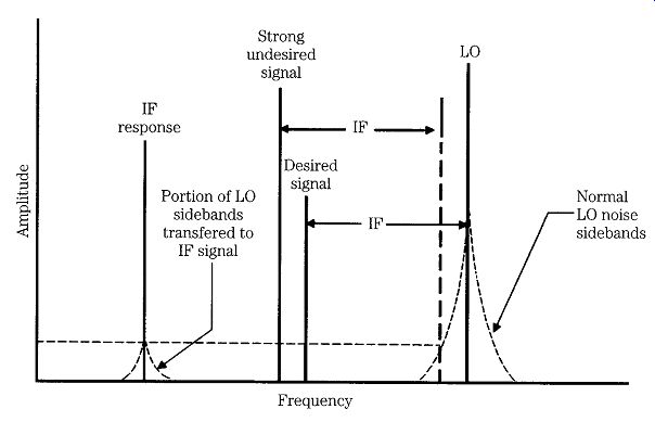
FIG. 21 Reciprocal mixing phenomenon: (A) LO with noise sidebands, desired
signal, and a strong undesired signal; (B) transfer of noise sidebands to
IF signal.
Reciprocal mixing occurs when noise sidebands from the local oscillator (LO) signal in a superheterodyne receiver mix with a strong undesired signal that is close to the desired signal. Every oscillator signal produces noise, and that noise tends to amplitude modulate the oscillator's output signal. It will thus form sidebands on either side of the LO signal. The production of phase noise in all LOs is well-known, but in more-recent designs the digitally produced synthesized LOs are prone to additional noise elements as well. The noise is usually measured in -dBc (decibels below carrier, or, in this case, dB below the LO output level).
In a superheterodyne receiver, the LO beats with the desired signal to produce an intermediate frequency (IF) equal to either the sum (LO + RF) or difference (LO - RF). If a strong unwanted signal is present then it might mix with the noise sidebands of the LO to reproduce the noise spectrum at the IF frequency (see Fig. 21). In the usual test scenario, the reciprocal mixing is defined as the level of the unwanted signal (dB) at 20 kHz required to produce noise sidebands 20 down from the desired IF signal in a specified bandwidth (usually 3 kHz on HF receivers). Figures of 90 dBc or better are considered good.
The importance of the reciprocal mixing specification is that it can seriously deteriorate the observed selectivity of the receiver, yet is not detected in the normal static measurements made of selectivity (it is a "dynamic selectivity" problem).
When the LO noise sidebands appear in the IF, the distant frequency attenuation (20 kHz off-center of a 3-kHz bandwidth filter) can deteriorate 20 to 40 dB.
The reciprocal mixing performance of receivers can be improved by eliminating the noise from the oscillator signal. Although this sounds simple, in practice it is often quite difficult. A tactic that will work well, at least for those designing their own receiver, is to add high-Q filtering between the LO output and the mixer input.
The narrow bandwidth of the high-Q filter prevents excessive noise sidebands from getting to the mixer. Although this sounds like quite the easy solution, as they say "the devil's in the details." Other important specifications IF notch rejection If two signals fall within the passband of a receiver they will both compete to be heard. They will also heterodyne together in the detector stage, producing an audio tone equal to their carrier frequency difference. For example, suppose we have an AM receiver with a 5-kHz bandwidth and a 455 kHz IF. If two signals appear on the band such that one appears at an IF of 456 kHz and the other is at 454 kHz, then both are within the receiver passband and both will be heard in the output. However, the 2-kHz difference in their carrier frequency will produce a 2-kHz heterodyne audio tone difference signal in the output of the AM detector.
In some receivers, a tunable, high-Q (narrow and deep) notch filter is in the IF amplifier circuit. This tunable filter can be turned on and then adjusted to attenuate the unwanted interfering signal, reducing the irritating heterodyne. Attenuation figures for good receivers vary from _35 to _65 dB or so (the more negative the better).
There are some tradeoffs in notch filter design. First, the notch filter Q is more easily achieved at low-IF frequencies (such as 50 to 500 kHz) than at high-IF frequencies (e.g., 9 MHz and up). Also, the higher the Q the better the attenuation of the undesired squeal but the touchier it is to tune. Some happy middle ground be tween the irritating squeal and the touchy tune is mandated here.
Some receivers use audio filters rather than IF filters to help reduce the heterodyne squeal. In the AM broadcast band, channel spacing is typically 10 kHz, and the transmitted audio bandwidth (hence the sidebands) are 5 kHz. Designers of AM BCB receivers usually insert an RC low-pass filter with a _3-dB point just above 4 or 5 kHz right after the detector in order to suppress the 10-kHz hetero dyne. This RC filter is called a tweet filter in the slang of the electronic service/ repair trade.
Another audio approach is to sharply limit the bandpass of the audio amplifiers.
For AM BCB reception, a 5-kHz bandpass is sufficient, so the frequencies higher can be rolled off at a fast rate in order to produce only a small response an octave higher (10 kHz). In shortwave receivers, this option is weaker because the station channels are typically 5 kHz, and many don't bother to honor the official channels anyway.
And on the amateur radio bands frequency selection is a perpetually changing ad hocracy, at best. Although the shortwave bands typically only need 3-kHz bandwidth for communications, and 5 kHz for broadcast, the tweet filter and audio roll-off might not be sufficient. In receivers that lack an effective IF notch filter, an audio notch filter can be provided. This accessory can even be added after the fact (as an outboard accessory) once you own the receiver.
Internal spurii
All receivers produce a number of internal spurious signals that sometimes interfere with the operation. Both old and modern receivers have spurious signals from assorted high-order mixer products, power-supply harmonics, parasitic oscillations, and a host of other sources. Newer receivers with either (or both) synthesized local oscillators and digital frequency readouts produce noise and spurious signals in abundance. (Note: low-power digital chips with slower rise times-CMOS, NMOS, etc.-are generally much cleaner than higher-power, fast-rise-time chips like TTL devices).
With appropriate filtering and shielding, it is possible to hold the "spurs" down to _100 dB relative to the main maximum signal output or within about 3 dB or the noise floor, whichever is lower.
A writer of shortwave books (Helms, 1994) has several high-quality receivers, including tube models and modern synthesized models. His comparisons of basic spur/noise level was something of a surprise. A high-quality tube receiver from the 1960s appeared to have a lower noise floor than the modern receivers. Helms attributed the difference to the internal spurs from the digital circuitry used in the modern receivers.
Receiver improvement strategies
There are several strategies that can improve the performance of a receiver.
Some of them are available for after-market use with existing receivers and others are only practical when designing a new receiver.
One method for preventing dynamic effects is to reduce the signal level applied to the input of the receiver at all frequencies. A front-end attenuator will help here.
Indeed, many modern receivers have a switchable attenuator built in to the front end circuitry. This attenuator will reduce the level of all signals, backing the largest away from the compression point and, in the process, eliminating many of these dynamic problems.
Another method is to prevent the signal from ever reaching the receiver front end. This goal can be achieved by using any of several tunable filters, bandpass filters, high-pass filters, or low-pass filters (as appropriate) ahead of the receiver front end. These filters might not help if the intermodulation products fall close to the desired frequency but otherwise are quite useful.
When designing a receiver project there are some things that can be done. If an RF amplifier is used then use either field-effect transistors (MOSFETs are popular) or a relatively high-powered bipolar (NPN or PNP) transistor intended for cable-TV applications, such as the 2N5109 or MRF-586. Gain in the RF amplifier should be kept minimal (4 to 8 dB). It is also useful to design the RF amplifier with as high a dc power-supply potential as possible. That tactic allows a lot of "head room" as input signals become larger.
You might also wish to consider deleting the RF amplifier altogether. One design philosophy holds that one should use a high-dynamic range mixer with only input tuning or sub-octave filters between the antenna connector and the mixer's RF input.
It is possible to achieve noise figures of 10 dB or so using this approach, and that is sufficient for HF work (although it might be marginal for VHF and up). The tube design 1960s vintage Squires-Sanders SS-1 receiver used this approach. The front end mixer tube was the 7360 double-balanced mixer.
The mixer in a newly designed receiver project should be a high-dynamic range type regardless of whether an RF amplifier is used. Popular with some designers is the double-balanced switching-type mixer (Makhinson, 1993). Although examples can be fabricated from MOSFET transistors and MOS digital switches, there are also some IC versions on the market that are intended as MOSFET switching mixers. If you opt for diode mixers then consult a source, such as Mini-Circuits (1992) for DBMs, that operate up to RF levels of _20 dBm.
Anyone contemplating the design of a high dynamic-range receiver will want to consult Makhinson (1993) and DeMaw (1976) for design ideas before starting.
References
Carr, J. J. (1994). "Be a Radio Science Observer-Part 1." Shortwave, November, pp. 32-36.
Carr, J. J. (1994). "Be a Radio Science Observer-Part 2." Shortwave, December, pp. 36-44.
Carr, J. J. (1995). "Be a Radio Science Observer-Part 3." Shortwave, January, pp. 40-44.
DeMaw, D. (1976). "His Eminence-The Receiver Part 1." QST, June, American Radio Relay League ( Newington, CT, USA), p. 27ff.
DeMaw, D. (1976). "His Eminence-The Receiver Part 2." QST, July, American Radio Relay League ( Newington, CT, USA), p. 14ff.
Dyer, J. A. (1993). "Receiver Performance: Descriptions and Definitions of Each Performance Parameter." Communications Quarterly, Summer, pp. 73-88.
Gruber, M. (1992). "Synchronous Detection of AM Signals: What Is It and How Does It Work?" QEX, September, pp. 9-16.
Helms, H. (1994). Author of All About Ham Radio and Shortwave Listeners Guide. Solana Beach, CA: HighText Publications, Inc. Personal telephone con versation.
Kinley, R. H. (1985). Standard Radio Communications Manual: With Instru mentation and Testing Techniques. Englewood Cliffs, NJ, USA: Prentice-Hall.
Kleine, G. (1995). "Parameters of MMIC Wideband RF Amplifiers," Elektor Electronics ( UK), February, pp. 58-60.
Magne, L. and Sherwood, J. R. (1987). How To Interpret Receiver Specifications and Lab Tests, A Radio Database International White Paper, Edition 2.0, 18 Feb, International Broadcasting Services, Ltd., Penn's Park, PA.
Makhinson, J. (1993). "A High Dynamic Range MF/HF Receiver Front-End." QST, February, pp. 23-28.
Mini-Circuits RF/IF Designers Handbook. Mini-Circuits ( P.O. Box 350166, Brooklyn, NY 11235-0003, USA. In UK: Mini-Circuits/Dale, Ltd., Dale House, Wharf Road, Frimley Green, Camberley, Surry, GU16 6LF, England).
Poole, I. (1995). G3YWX, "Specification-The Mysteries Explained," Practical Wireless, April, p. 41.
Poole, I. (1995). G3YWX, "Specification-The Mysteries Explained," Practical Wireless, March, p. 57.
Rohde, U. L., and Bucher, T. T. N. (1998). Communications Receivers: Principles & Design. New York: McGraw-Hill.
Tsui, J. B. (1985). Microwave Receivers and Related Components. Los Altos, CA: Peninsula.