AMAZON multi-meters discounts AMAZON oscilloscope discounts
The basic function of differential voltmeters or differential voltage measuring is to apply an unknown voltage against one that is accurately known, and to measure the difference between the two on an indicating device. If the known voltage is adjusted to the exact potential of the unknown voltage, one can determine the unknown quantity being measured as accurately as the known voltage (or reference standard). A typical differential voltage measurement is shown in Fig. 2-1.
The null meter (Mx) indicates when the voltage (Eae) at the potentiometer is equal to the unknown voltage, Ex. By considering the ratio of resistances Rab and Rae in the potentiometer, the ratio of Ene to the known reference voltage (Eref) may be determined precisely.
The potentiometric method of voltage measurement is highly accurate since precise resistance ratios can be determined. No current is drawn from either the standard cell or the unknown voltage source at null. The source impedance, Rx, therefore does not affect measurement. The divider output tap (b) is adjusted to null Erer.
The potentiometric method of voltage measurement (see Fig. 2-1) can be represented by the equation where,
E Rae Ex = rer R ab Ex is the unknown voltage,
Erer is the reference voltage,
Rae is the full potentiometer resistance,
Rab is the potentiometer resistance from slider to one end.
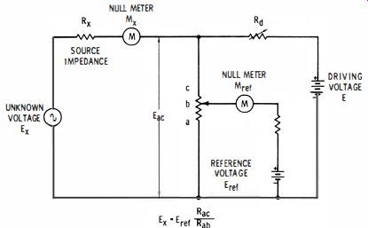
Fig. 2-1. Potentiometer method of measuring unknown voltages.
For example, if the reference voltage were 5 volts, the total potentiometer resistance 1000 ohms, and the slider resistance for null 200 ohms, then 200 Ex = 5 1000 or 1 5 X"5 = 1 volt
BASIC OPERATING PRINCIPLES
Fig. 2-2 illustrates a simplified, conventional differential voltmeter in which the potentiometer slider has been replaced by a Kelvin
Varley divider, and the driving or source voltage E has been replaced by an accurate supply, E" referenced to a standard voltage Erer
In practice, the null device is a solid-state voltmeter rather than a galvanometer.
Using the method shown in Fig. 2-2, a high-voltage standard is necessary to measure high voltages. This need may be overcome by inserting a voltage divider between the source and the null-meter circuit. However, this practice provides a relatively low input impedance for voltages that are higher than the reference standard.
This low input impedance is undesirable; accurate measurements can not be obtained if current is drawn from the source that is being measured. Most differential voltmeters used today offer an impedance approaching infinity only at null condition and then only if an input voltage divider is not used.
One way to eliminate this problem is to isolate the measuring circuits from the input by an amplifier. Such an arrangement provides a high input impedance which eliminates loading the source, resulting in a differential voltmeter whose input impedance is independent of both null condition and range.
Differential voltmeters are often combined with d-c voltage standards. This approach produces one package that provides several benefits for making precision voltage measurements.
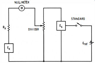
Fig. 2-2. Simplified convention.1 differenti.1 voltmeter.
TYPICAL DIFFERENTIAL VOLTMETER OPERATION
Fig. 2-3 is a block diagram of a differential voltmeter that has been combined with a d-c voltage standard and includes an isolating amplifier at its input. The circuit also has an a-c/d-c converter that permits it to make differential measurements on a-c voltages (by precise conversion of the unknown a-c voltage to an equivalent d-c voltage) and to serve as a precision a-c voltmeter.
When a voltage to be measured is applied to the input terminals, the amplifier responds by re-creating this voltage at the summing point inherently balancing the system to achieve a constant, high input impedance. The amplifier output is converted to a 1-volt level by means of a precision range divider switch for direct comparison with a 1-volt internal reference. The range switch performs two operations. First, it changes the overall feedback factor and thus the overall amplifier gain. Second, the range switch selects the potentiometer tap on the range stick. Consequently, the choice of the proper range enables any input voltage between a and 1000 volts to be represented by a proportional voltage between 0 and 1-volt at the tap connecting to the potentiometer.
The isolation stage consists of a series-connected pair of amplifiers, a low-level chopper-stabilized amplifier, and a high-voltage amplifier.
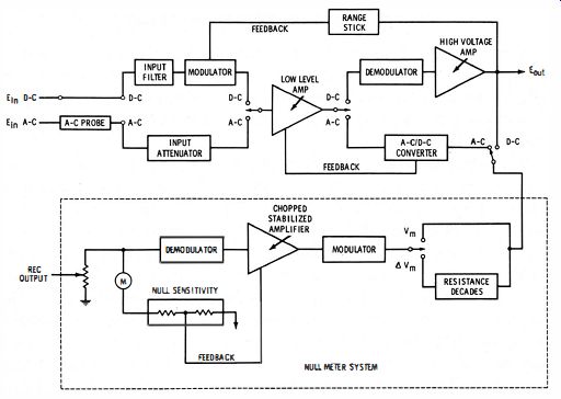
Fig. 2-3. Block diagram of an a-c/d-c differential voltmeter.
The high level of feedback (over 100 db) ensures gain accuracy and produces a high input impedance (over 1000 megohms). The a-c probe is used with a-c measurements. The unknown a-c signal is fed from the precision attenuator to the high-impedance, low-level amplifier. It is then amplified and applied to a diode bridge whose half-wave signal is averaged to produce a d-c output. The d-c output of the converter is measured in the same manner as the d-c different mode-by connecting the null-meter decade divider system.
Consequently, the a-c measurement is made with a high degree of accuracy, since the a-c signal is converted to d-c and measured with the same precision dividers and reference standard used in d-c operation. With this method, accuracy can approach that of the d-c mode.
The differential voltmeter can be converted into a d-c standard by means of a front panel control. The same feedback amplifier and range stick are used. However, the internal reference supply now becomes the input to this amplifier. The input is automatically nulled against a feedback voltage which is determined by the range-switch setting and the output voltage at the sensing terminals. A range switch on the decade divider is mechanically linked to a voltage divider connected to the input of the null meter. This vernier provides the fifth and sixth digits of resolution.
COMMON-MODE SIGNAL PROBLEMS
One of the problems in any voltmeter-especially in those designed for precision measurements such as differential voltmeters-is an effect known as common-mode insertion. Therefore, in any precision laboratory-type meter, the common-mode rejection factor becomes an important characteristic.
To understand the common mode problem, assume that we have an instrument with two input terminals, 1 and 2. The instrument ideally responds to the voltage between terminals 1 and 2. This voltage is called the differential voltage. If terminal 1 is at +0. 1 volts and terminal 2 is at -0. 1 volts, the differential voltage applied to the instrument is 0.2 volts. Again, if terminal 1 is at + 1 0.0 volts and terminal 2 is at + 10.0 volts, the differential voltage applied to the instrument is zero, and the instrument should respond accordingly.
In certain situations, however, when equal + 10-volt input signals are applied, the instrument will not respond as if the differential voltage were zero. That is, the instrument's output will indicate that a differential voltage is present. It is apparent that the application of + 10 volts to both input terminals may in some way adversely affect operation of the instrument. The + 10-volt signal is called the common-mode voltage since is it common to both input terminals in terms of amplitude, polarity, and time.
While d-c voltages have been used in the preceding discussion, the same treatment applies for alternating current. Since any voltmeter should ideally respond only to differential voltages, it should ignore the common-mode voltage. The means by which a common-mode voltage may affect an instrument is best shown by means of an example. A typical instrumentation set (simplified) is shown in Fig. 2-4. A transducer (typically a welded thermocouple) is connected to a remotely located instrument (containing a d-c amplifier.) As shown, a signal voltage causes a signal current to flow in the input resistance via the transducer internal resistances (R1, R2). The instrument has an impedance (Z) to local ground (earth or rack ground). A common-mode voltage exists between local and transducer grounds. The common-mode voltage exists between local and transducer grounds. The common-mode voltage causes a common-mode current to flow through the transducer internal resistances and then through the impedance of the instrument to local ground via the signal leads. It can be seen that the common-mode current is intermingled with the signal current and thus causes a spurious signal-current to flow through the instrument's input resistance. This spurious signal current is a source of error.
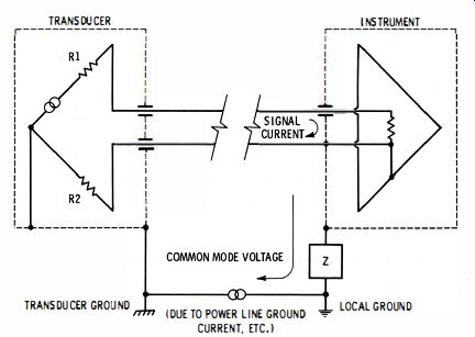
Fig. 2-4. Common mode signal insertion.
Capacity of an instrument to reject a common-mode signal and thus reduce the spurious signal current is called common-mode rejection (cmr). Cmr is usually specified in db at some frequency or range of frequencies, for example, 130 db minimum at 60 hz. This means that the spurious signal effect of a given common-mode signal is reduced by 130 db or more. For example, the effect of 100-volt, 60 hz, common-mode signal is reduced to that of a 33-p.v maximum equivalent signal. It may be said that a 100-volt, 60- hz, common-mode signal results in a 33-p.v maximum differential signal.
One of the major sources of common-mode signals is induced ground currents, usually at the a-c power-line frequency. These signals can generate a potential of several volts between the signal source ground and the 'chassis ground. Unless shunted, these currents will cause a voltage to appear at the input or output which can be larger than the signal itself, resulting in an erroneous reading or output voltage. In differential voltmeters and many digital meters (especially those having a differential or comparison circuit) the input and output terminals are often "floating." That is, they are mounted separately from the main chassis. Any a-c voltages present at these terminals can be rejected by means of a circuit ground.
Such a circuit is shown in Fig. 2-5. This circuit is used by Hewlett-Packard in the Model 740A, which is both a d-c standard and a differential voltmeter. As shown, the negative terminals of both input and output are connected together. The output negative terminal is connected to the chassis through capacitor C1. The input negative terminal is connected to the guard shield (a metal enclosure around the floating terminals) through capacitor C2. In turn, the guard shield and chassis are connected by capacitor C3. This shunts any a-c potentials that may exist between the terminals and chassis, terminals and guard, or guard and chassis.
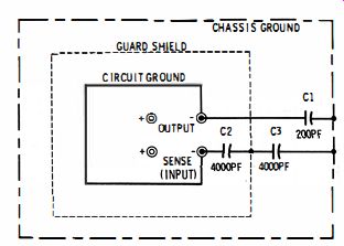
Fig. 2-5. Guard system used in Hewlett-Packard Model 740C.
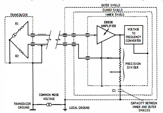
Fig. 2-6. Guard system used in n Vid Model 510.
Another guard circuit used by Vidar, Inc. in their Model 510 is shown in Fig. 2-6. A comparison of this setup with the arrangement shown in Fig. 2-4 reveals that the common-mode path has been broken by means of . the partitioning between the inner and outer shields (the instrument proper is enclosed by the guard shield.) In this way the instrument-to-local-ground impedance (shown as Z in Fig. 2-4) has been raised to a very high value. The effect of raising the instrument to local ground impedance is to reduce the spurious signal current due to the common-mode voltage. The higher the instrument-to-local-ground impedance is, the lower is the spurious signal current.
It should be noted that the instrument-to-local-ground impedance consists primarily of the small (but not negligible) capacitance between the inner and outer shields. This means that the instrument-to-local-ground impedance will be a function of frequency and that the common-mode rejection will be a function of frequency-the common mode rejection decreasing by 6 db per octave as the common-mode signal frequency increases.
In most cases, this effect does not pose a problem, since the predominant common-mode signal usually occurs at line frequency (50/60 hz).