AMAZON multi-meters discounts AMAZON oscilloscope discounts
The conventional shop-type vom and vtvm are analog meters. That is, they use rectifiers, amplifiers, and other circuits to generate a current proportional to the quantity being measured. This current, in turn, drives a meter movement. Laboratory-type analog meters also operate in this manner. However, laboratory meters include many circuit refinements to improve their accuracy and stability. Many of the special-purpose analog meter circuits are unique to laboratory equipment. This section describes the basic principles of analog meters and shows how these basic principles are adapted to laboratory use.
METER MOVEMENTS AND SCALES
The meter movements in most shop-type equipment consist of a pointer attached to a coil supported by pivots and jewels. In high-accuracy meters, a taut-band suspension is substituted in place of pivots and jewels. The moving coil in the taut-band meter mechanism is suspended on a platinum-alloy ribbon, eliminating friction and problems concerning repeated measurements. In order to eliminate tracking error on mass-produced meters, the meter faces are custom-calibrated and photographically printed to match exactly the linearity characteristics of each individual meter movement at all points. By combining taut-band suspension with custom-calibrated scales, the chance for mechanical error is kept to an absolute minimum.
BASIC DC MEASUREMENTS
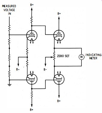
Fig. 3-1 . Basic doc vacuum-tube voltmeter circuit.
The d-c voltmeter represents a straightforward application of electronics to measuring instruments. In laboratory work, d-c voltages are usually measured by a vtvm rather than a vom. Most vtvm's have a direct-coupled amplifier preceding the meter movement. Fig. 3-1 is a basic vtvm circuit for measurement of d-c voltage. The amplifier performs two important functions. First, it increases the input impedance of the meter so that the instrument draws negligible current from the circuit under test. Because of the amplifier the electronic voltmeter is a voltage-operated device, whereas the simple meter movement (vom) is a current-operated device. This distinction is important, since the voltage in many circuits can be altered by the current required for operating a meter movement alone.
A second amplifier function is to increase the effective sensitivity of the meter movement. An amplifier changes the measured quantity into a current of sufficient magnitude to deflect the meter movement.
An amplifier also limits the maximum current applied to the meter movement. Therefore, there is little danger that unexpected overloads will burn out the meter movement.
ELIMINATING DRIFT
One of the problems common to the basic vtvm circuit is drift. This is especially aggravated on low-level measurements. A widely used technique for eliminating drift in such low-level measurements is to convert the d-c signal into a comparable a-c signal by alternately applying and removing the d-c signal. The resulting "chopped" signal is amplified in a-c amplifiers and then synchronously rectified at a high level for operating the meter movement. Overall d-c feedback ensures accuracy of the d-c gain. Therefore, d-c drift is limited to a value set by the input chopper. The photoconductive chopper is often used in precision laboratory-type electronic voltmeters. In such a circuit the d-c signal is converted to a comparable a-c signal by illuminating a group of photoconductive or photosensitive resistors periodically. This results in a low-noise, high-impedance chopper action.
AUTOMATIC RANGING CIRCUITS
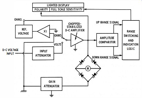
Fig. 3-2. Block diagram of Hewlett-Packard Model 414A automatic ranging voltmeter.
Automatic ranging is usually limited to digital meters. The great majority of analog meters (including most laboratory equipment) require that the scales be changed manually for measurements that vary widely. However, it is possible to combine the touch-and-read convenience of a digital meter with the economy of an analog instrument. With such a circuit, both range changing and polarity selection are automatic. This provides rapid "hands free" measurement of both voltage and resistance. Such a circuit is shown in Fig. 3-2. A chopper-stabilizer d-c amplifier, input attenuator, gain attenuator, and metering circuit form the basic circuit. Range-changing decisions are indicated by means of a lighted display and are based on two signal levels, one near full scale on a given range and the other at one-fourth of full scale. An amplitude comparator produces an "up-ranging signal" whenever the input voltage tends to rise above the level which is near full scale and a "down-ranging signal" whenever the input voltage tends to fall below the level near one-fourth of full scale. Range switching and indicating logic are a set of four multivibrators which define the twelve ranges of the instrument.
BASIC DC CURRENT MEASUREMENTS
In the basic vom the meter movement (by itself) serves the purpose of measuring appreciable amounts of direct current. In these cases the meter coil requires relatively few turns to generate sufficient magnetic flux for deflecting the meter pointer. For lower current measurements the sensitivity of the meter movement must be increased, usually by using more turns in the coil. These added turns increase the resistance of the current path. This can be troublesome in low-impedance circuits. The laboratory-type electronic current measuring instruments overcome this difficulty by measuring the small voltage drop across a low-value resistance placed in series with the current to be measured. Most laboratory meters are equipped with internal, calibrated, shunt resistors for reading direct currents, in this way, without accessory equipment.
CLIP-ON METERS
Current measurements using a series resistor have the obvious disadvantage of interrupting the circuit under test. In many applications, insertion of a resistance in the current path may alter the current being measured or even alter the circuit operation. To overcome this difficulty, clip-on milli-ammeters use current probes which simply clip around the current-carrying wire and measure direct currents.
A typical clip-on meter will measure currents from 0.1 milliampere to 10 amperes.
These probes use the second-harmonic flux-gate principle to sense magnetic flux around the wire. (See Fig. 3-3.) The probe encircles the wire with a magnetic core which is saturated periodically by a 20- khz driving current. Saturation interrupts the magnetic circuit, effectively "gating" any flux induced in the core by current in the wire.
This gated a-c flux couples with sensing coils on the core, inducing a 40- khz voltage proportional to the current in the wire. The circuitry amplifies the coil voltage and drives the indicating meter accordingly.
High linearity is achieved by using negative d-c feedback current, balancing the input ampere-turns against the feedback ampere-turns.
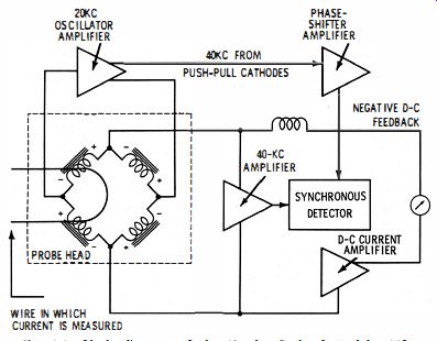
Fig. 3-3. Block diagram of the Hewlett-Packard Model 428B clip-on type probe.
The clip-on probes are finding wide use in solid-state circuit measurements where current has to be monitored carefully. Sensitivity is such that base current can be measured. There are a variety of other uses, such as measuring the current in ground loops; where the impedance is too low for the series-resistance technique to be applied.
A unique feature of these probes is that the sums and differences of currents in several wires can be determined by running the wires through the probe at the same time. This technique is useful for balancing push-pull amplifier stages : run the two plate leads in opposite directions through the probe and then adjust for a null on the current meter.
The probes allow current measurements in large-dimension conductors such as pipes, multiconductor cables, lead-sheathed cables, or microwave waveguides. With large aperture probes, difficult-to-measure quantities, such as corrosion current in small structural members and circulating direct current and low-frequency alternating current in ground straps and waveguides, can easily be determined.
RESISTANCE MEASUREMENTS
Resistance is usually determined through the familiar form of Ohm's law, E = JR. In simple vom's this is done by applying a known voltage (E) to the unknown resistance (R) and then measuring the current (I) passing through it. With E and I known, R can be computed. In actual practice, computation is unnecessary since the resistance scale of the meter is pre-computed.
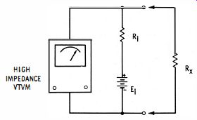
Fig. 3-4. Circuit for making nominal resistance measurements with an electronic
voltmeter.
Laboratory-type electronic voltmeters use a modified procedure for resistance measurement. As shown in Fig. 3-4, the current in the circuit depends on the series combination of the unknown resistor (Rx) and the internal resistor (R1) . This means that both the voltage and current in the external circuit will change according to the value of the unknown. The resistance scales of the meter are calibrated for the measurement of this unknown resistance.
If Rx were infinite, the meter would read the full battery voltage (E1). Full-scale deflection, therefore, would correspond to a resistance of infinity. If Rx were zero (short circuit), the meter would read zero.
The mid-scale range occurs when Rx equals R1
The resistance Rh included as part of the ohmmeter circuit, provides a convenient means of changing the range of the instrument. When values of low resistance are being measured, the finite resistance of the ohmmeter leads-included in the total resistance measurement can contribute considerable error. To meet this problem the circuit can be altered so that the resistance of the current-carrying leads is calibrated as part of Rh while the resistance in the voltmeter leads is insignificant compared with the high input impedance of the metering circuit. Such a circuit is shown in Fig. 3-5.
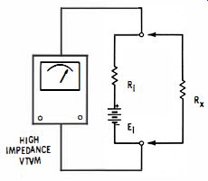
Fig. 3-5. Circuit for measuring low Rx value resistance.
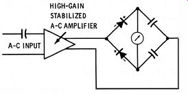
Fig. 3-6. Circuit for average responding voltmeter.
An external power source is often used in laboratory work where it is necessary to measure very high or very low resistances. For very high resistances a high voltage is applied to the unknown, and the current is measured on a sensitive current meter. High-resistance measurements can be disturbed by the impedance of the measuring voltmeter when this impedance is comparable to the resistance being measured. Many laboratory meters account for this by adjusting the value of R1 on the high-resistance ranges to compensate for the voltmeter input impedance. For example, on a 100-megohm scale the value of R1 is actually 200 megohms. The parallel combination of the 200-megohm R1 and the 200-megohm input impedance of the meter gives an effective internal impedance of 100 megohms.
To measure extremely low resistances such as those found in short lengths of large wire or in relay contacts, a constant-current source may be used to supply a fixed amount of current through the unknown resistance. A sensitive voltmeter is then used to measure the voltage drop across the resistance being measured. With this combination, resistance measurement as low as one micro-ohm may be made.
BASIC A-C VOLTAGE MEASUREMENTS
Electronic instruments for measuring a-c voltages also use an amplifier with the meter movement, but add a rectifier circuit to convert the alternating current to direct current. Most shop-type vom and vtvm units are rms-reading instruments. Mathematically, the root-mean-square (rms) value of any complex quantity is obtained by adding the squares of each component and then taking the square root of this sum. Laboratory-type meters, however, fall into three broad categories : average-responding, peak-responding, and rms responding.
The circuit principle of the average-responding meter is shown in Fig. 3-6. Here, the a-c signal is amplified in a gain-stabilized a-c amplifier and then is rectified by the diodes. The resulting current pulses drive the meter. The meter deflection is proportional to the average value of the waveform being measured.
The peak-responding voltmeter shown in Fig. 3-7 places the rectifier in the input circuit where it charges the small input capacitor to the peak value of the input signal. This voltage is passed to a d-c amplifier which drives the meter. Meter deflection is proportional to the peak amplitude of the input waveform.
Both of these meters (average-responding and peak-responding) have scales calibrated such that the rms value of a sine-wave input voltage is indicated, since the meters are used primarily for sine-wave measurements. Therefore, the average-responding type reads 1.11 times higher than the average voltage, while the peak-responding type indicates 0.707 of the peak value. Consequently, both meters may be in error if the measured signal is not a pure sine wave. The amplitude and phase of the harmonics present affect the peak and average values of the waveform, upsetting the rms calibration. The average reading voltmeter is not affected by distortion as much as the peak reading type. However, if highly complex waveforms are measured, then a true rms-responding voltmeter is recommended.
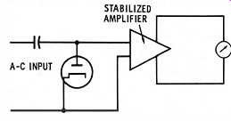
Fig. 3-7. Circuit for peak responding voltmeter.
For general laboratory work the average-responding voltmeter is used extensively, since it is less affected by distortion of the waveform.
Peak-responding meters are used for higher-frequency measurements because of their lower input capacitance. The capacitance to ground of the input circuit and probe of a voltmeter must be included as part of the input impedance. This capacitance acts as a high-frequency bypass to the input resistance and limits the frequency range of most a-c voltmeters.
Since the diode rectifier of peak-responding voltmeters is placed in the probe tip preceding the amplifier, shortening the signal path, the a-c capacitance is low. Input capacitances of one to three picofarads are characteristics of those instruments. The extension of this technique into the low-voltage (millivolt) range is impractical because of the nonlinear response of diodes at low signal levels. A variation of the rectifying technique is required to eliminate the diode nonlinearity. Usually, this is accomplished by using two diodes.
TRUE RMS-RESPONDING VOLTMETERS
Complex waveforms are measured most accurately by an rms responding voltmeter. In laboratory instruments this is performed by sensing the heating power of the waveform which is proportional to (Erlll')?' The indicating circuitry responds to the square root of the heating power. Heating power is measured by feeding an amplified version of an input waveform to the heater of a thermocouple, the voltage output of which is proportional to the heating power of the waveform.
One of the major problems in this technique is the nonlinear behavior of the thermocouple, as well as slow response and possible burnout of the thermocouple. These factors complicate calibration of the indicating meter. This difficulty can be overcome by the use of two thermocouples mounted in the same thermal environment. Nonlinear effects in the measuring thermocouple are cancelled by similar nonlinear operations of the second thermocouple.
As shown in Fig. 3-8, the amplified input signal is applied to the measuring thermocouple, and a d-c feedback voltage is fed to the balancing thermocouple. The d-c voltage is derived from the voltage output difference between the thermocouples. The circuitry may be looked upon as a feedback control system which matches the heating power of the d-c feedback voltage to the input waveform heating which, in turn, is proportional to the rms of the input signal. Therefore, the meter indication is linear.
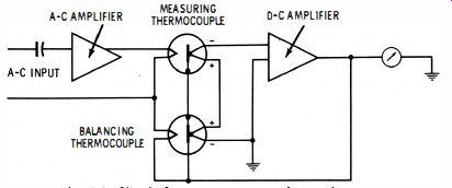
Fig. 3-8. Circuit for true rms-responding voltmeter.
THE SAMPLING VOLTMETER
(A) Waveform of input signal. (B) Waveform of a collection of signals. (C) Waveform of signals after mixing.
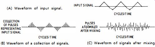
Fig. 3-9. Incoherent sampling technique.
The sampling voltmeter is used to measure complex or nonsinusoidal signals. There are several types of sampling voltmeters; one of the most effective uses the incoherent sampling technique. This is particularly useful where the waveforms have large crests such as sawtooth or triangular waves.
The incoherent sampling technique is illustrated in Fig. 3-9. The technique is best explained by representing each sample with a pulse whose height is proportional to the amplitude of the input signal at the instant the sample is taken. The average, rms, or peak value of the collection of pulses in Fig. 3-9B differs from the input signal (Fig. 3-9A) only by a scale factor. Suppose that these pulses are collected and scrambled. The order in which the pulses appear after being scrambled together results in a waveform similar to that of Fig. 3-9C. Since the pulses are the same, the average, rms, and peak values of this rearranged waveform are identical to the average, rms, and peak values of the waveform in Fig. 3-9B.
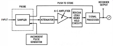
Fig. 3-10. Block diagram of a Hewlett-Packard Model 3406A sampling voltmeter.
Fig. 3-10 is a block diagram of such a voltmeter. Samples taken in the probe are pulsed by the incoherent pulse generator in the sampler. These pulsed samples are fed through the attenuators and amplifiers to the "boxcar" (zero-order hold) circuit. The hold circuit stores each sample until the next sample is taken. The output of the boxcar circuit is available directly. This output may be used to obtain true rms measurements when used with an rms voltmeter or for peak measurements when used with a peak-reading voltmeter. The output of the boxcar circuit is also fed to a special signal processor which contains noise-suppression circuits for low signal ranges. Low-strength signals mixed with noise of equal or near-equal strength will produce inaccurate readings.