High Frequency Components [Electronic Component Tests & Measurements (1963)]

Tests of high-frequency components have the same theoretical foundation as tests of components operating at comparatively low frequencies. However, the practical aspects differ considerably and justify treatment in a separate section.

For example, consider the problem of measuring AC resistance at 20 mhz. An AC Wheatstone bridge is commonly utilized, but its construction and range differs considerably from a 1- khz Wheatstone bridge. First, stray capacitance must be minimized in the bridge design because at 20 mhz, 10 mmf stray capacitance has a reactance of only 800 ohms. Compare this value with a reactance of 16 megohms at 1 khz. Stray capacitance unbalances a bridge and prevents indication of a proper null.

When stray capacitance is minimized, its effects are still sufficiently objectionable in simple bridges that a top resistance indication of 600 ohms is provided. Although the measurement range is comparatively limited, a simple HF Wheatstone bridge finds considerable use in practical work. If higher values of AC resistance need to be measured, indirect methods are necessarily employed. IF and RF sweep generators provide practical in-circuit tests of high-frequency components. Excessive AC resistance in a plate-load coil, for example, shows up as abnormal bandwidth.

Inductance measurements at high frequencies are usually made indirectly. An accurately calibrated grid-dip meter may be employed. The distributed capacitance of the coil is first measured, as explained subsequently. When the distributed capacitance is known, the total shunt capacitance in the test circuit is then known, and the grid-dip meter indicates the resonant frequency. In turn, L is the only unknown quantity in the standard resonant-frequency formula, from which the inductance value may be calculated. You will find a reactance and resonant-frequency slide rule very convenient, since the necessity for calculation is avoided. The Shure reactance slide rule costs only $1.00 and is satisfactory in practical work.

Note in passing that a Q-meter is a most useful instrument for testing high-frequency components. But its cost is comparatively high and is seldom profitable to a service shop.

However, when the need arises, you might be able to borrow a Q-meter from a nearby technical school or electronics factory. This instrument provides direct measurement of Q, L, R, and C at radio frequencies. Its operation is explained in most radio-engineering texts ; the interested reader may refer to these.

Ohm's law applies at high frequencies in exactly the same manner as it does at low frequencies. The differences are merely that inductances have comparatively small values in any high-frequency application ; stray and distributed capacitances cannot be neglected and may dominate component characteristics. The efficiency of a simple semiconductor diode may be entirely different at 40 mhz than at 1 khz. A resistor that has a value of 0.5 megohm at zero frequency will have a lower (sometimes very much lower) value at 100 mhz, and it will draw a leading current. Such considerations modify practical test procedures, and require suitable test setups.

HIGH-FREQUENCY RESISTANCE TESTS

High-frequency resistance cannot be measured with an ohmmeter. For example, a dipole antenna is shown in Fig. 1 (A). An ohmmeter measures an infinite terminal resistance, but when tested with an antenna-impedance meter at the self resonant frequency of the antenna, a terminal resistance of 72 ohms is measured. Again, the zero-frequency input resistance of the RF tuner depicted in Fig. 1 (B) is infinite, whereas its resonant-frequency input resistance is 300 ohms.

The DC input resistance of the tuner shown in Fig. 1 (C) is almost zero, although its on-channel input resistance is 300 ohms.

MEASUREMENT OF ANTENNA RESISTANCE

When the dipole antenna illustrated in Fig. 1 is driven at its self-resonant frequency, the input impedance is purely resistive ; the antenna "looks like" a pure high-frequency resistance at its terminals. However, when operated off its self-resonant frequency, the antenna terminal resistance is accompanied by either a capacitive or an inductive reactance. In other words, the antenna then has an input impedance, instead of a simple input resistance.

(A) DC resistance infinite; Hf resistance 72 ohms. (B) DC resistance infinite; HF resistance 300 ohms. (C) DC resistance near zero; HF resistance 300 ohms.

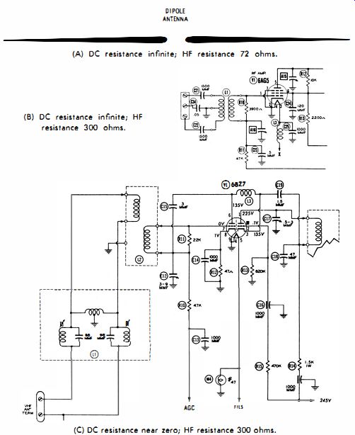
Fig. 1. High frequency resistance measurements.

The same general observation applies to the RF tuners in Fig. 1. The tuner input impedance is essentially a high frequency resistance on the channel to which the tuner is set, but when tested at an off-channel frequency, the input resistance of the tuner is accompanied by either inductive or capacitive reactance-and we must then consider the input impedance of the tuner. There has been some loose usage of the term "impedance" in the past, and the input resistance of an antenna or front end has been called an input impedance, although no reactance is present.

An antenna-impedance meter is a high-frequency bridge.

Unless the arms in a high-frequency bridge have comparatively low values, the bridge accuracy will be poor at high frequencies. This inaccuracy results from the bypassing action of stray capacitances around the bridge arms. However, since most antennas have a comparatively low input resistance or impedance, a bridge such as depicted in Fig. 2 can be used in most applications. This type of instrument is commonly called an antenna-impedance meter, although strictly speaking it is a high-frequency resistance bridge ; it does not measure impedance.

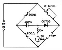
Fig. 2. Antenna impedance meter circuit.

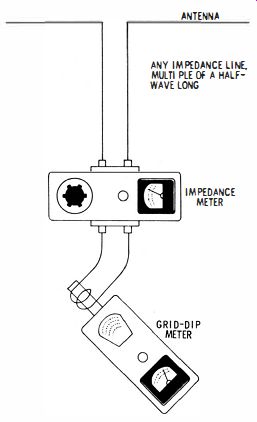
Fig. 3.

The bridge cannot be used to check DC resistance because the indicator is energized by an RF probe arrangement. One arm of the bridge is a calibrated potentiometer that is adjusted for a null-indication on the meter when a lead-in is connected across the Test terminals. The dial is calibrated from 10 to 600 ohms in a typical bridge. The bridge can be driven from any RF source having moderate output such as a grid-dip meter or RF signal generator with a high-level (1 volt ) output.

Test Procedure

A suitable test setup for measuring antenna resistance is shown in Fig. 3. The bridge can be connected directly to the antenna terminals if they are accessible. Otherwise, the bridge must be connected to the antenna via a lead-in. In the case of a half-wave dipole antenna with accessible terminals, a direct connection can then be made to the bridge. The bridge case is left floating (ungrounded ). A pickup loop can be used to drive the bridge, with a grid-dip meter as an AC source. The test frequency should be set in the vicinity of the half-wave resonant frequency of the antenna. To determine the approximate bridge-driving frequency, use the following formula :

f = 467.4 / length in feet

Set the grid-dip meter to this frequency. Then adjust the bridge for minimum indication on the meter--only a partial null can be anticipated at this time, and for a simple dipole antenna, the bridge reading will be less than 75 ohms. Now make back-and-forth adjustments of the bridge-driving frequency and the bridge dial to obtain a complete null (if possible ). In a case a complete null is obtained, the bridge then reads the antenna input resistance. Note that this method is not reliable at frequencies above 40 or 50 mhz, due to limitations of the bridge response as well as disturbances imposed by the proximity of the operator.

Cause of Incomplete Nulls

When a complete null cannot be obtained, the antenna-input resistance is actually an impedance-there is inductive or capacitive reactance present with the effective resistance. This situation is usually caused by partial resonances in nearby guy wires or other metallic objects. A metallic mast can also introduce a partial resonance coupled to the antenna. Guy wires should be split up into sections with insulators to throw their self-resonant frequencies out of range and permit a better null in the resistance test. The measured input resistance might be as low as 10 ohms, or as high as 100 ohms for a simple dipole antenna that is strongly affected by proximity of metal objects or wires. Even if the input resistance is purely resistive, the value will also vary with the dipole height above ground.

Test With Lead-In

When it is inconvenient to make the test directly at the antenna terminals, use a half-wave line between the bridge and the half-wave dipole. The question then arises concerning how to determine the electrical length of this half-wave line, inasmuch as the exact self-resonant frequency of the dipole is unknown. One method is to select the bridge-driving frequency by "guess-timation" and cut a half-wave line to this frequency.

If a complete null cannot be obtained because of a poor guess, the lead-in can be shortened or lengthened to accommodate a new bridge-driving frequency.

Electrical Length of Lead-In

Although the electrical length of a dipole can be calculated with comparative accuracy from its physical length, this is not always possible in the case of a lead-in. A dipole has air dielectric, whereas a lead-in often has a solid dielectric. Solid dielectric causes the electrical length to be greater than the physical length, how much depending on the type of dielectric ; so a quick method is needed for measuring the electrical length of a lead-in. To make the test, use a sample section of the lead-in, 10 or 15 feet in length. Short-circuit the conductors at one end and measure the resonant frequency of this quarter-wave stub, as illustrated in Fig. 4. (The grid-dip meter should be accurately calibrated.) Convert the measured frequency into its corresponding wavelength in meters. (One meter is equal to 39.37 inches. ) This divided by 4, gives the electrical length of the stub, since its electrical length is equal to 1f4 of the measured wavelength.

The velocity factor of the stub is equal to its physical length divided by its electrical length. The velocity factor is always less than 1. Knowing the velocity factor of the lead-in, you can cut it to exactly an electrical half-wavelength at the desired driving frequency.

Note that in case a half-wave lead-in is too short, you can use one wavelength, 11 wavelengths, 2 wavelengths, etc. The reason for these choices is that each half-wave length of lead-in repeats the load. In other words, the terminal impedance of the antenna is reflected exactly by each half-wavelength of lead-in. An example of velocity-factor measurement is as follows : A sample section of twin lead was measured and found to be 170.75 inches (or 4.33 meters) long physically. One end of the stub was shorted (with a copper plate) as shown in Fig. 4. Now, if the velocity factor were equal to 1, its resonant wavelength would be 4 x 4.33, or 17.32 meters. Its resonant frequency would be 300,000,000/17.32 = 17.3 mhz.

However, a grid-dip meter indicates a resonant frequency of 14 mhz. Therefore, the velocity factor is equal to 14/17.3, or 81 '7'0 .

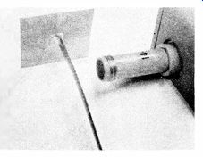
Fig. 4.

Interference in Bridge Test

Sometimes the bridge does not read zero, even though the driving voltage is removed when testing antenna resistance.

In this case, the antenna is usually picking up a strong signal that is interfering with the test. Orienting the dipole is helpful, although this is not always possible. Hence, it is occasionally necessary to wait for a quiet period to make antenna tests.

High-frequency bridges are often provided with an output jack, as depicted in Fig. 5. If you plug a pair of earphones into the bridge, you may be able to identify the interfering signal.

RESISTANCE OF A TRAP

The HF resistance of a trap, or any series-resonant LC device, can be measured easily with the bridge depicted in Fig. 2. Merely connect the trap across the bridge terminals (Fig. 3 ) instead of across the antenna. Tune the grid-dip meter to the approximate frequency of the trap. Then adjust the bridge for minimum indication. The grid-dip meter must then be readjusted to get a better null. Finally, by working back and forth, a complete null will be obtained. The bridge dial then indicates the HF resistance of the trap. An ideal trap would have zero resistance, but in practice there is appreciable resistance present, contributed principally by the coil.

Inasmuch as simple RF bridges can measure a top resistance of only 600 ohms, this method is generally unsuitable for measuring the resistance of parallel resonant units. Another limitation applies to tests of both series and parallel LC devices ; this type of bridge is not rated for test frequencies above 40 or 50 mhz. However, within its limitations, this is a very useful test method.

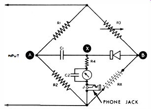
Fig. 5. Phone jack for earphones.

HIGH-FREQUENCY RESISTANCE OF A COIL

Inasmuch as the measured HF resistance of an LC trap is effectively the resistance of the coil, the series capacitance can be varied to test the coil at any frequency to which it can be resonated. Connect the coil under test in series with a variable capacitor, and set the grid-dip meter to the desired frequency. Measure the HF resistance as previously explained, except that in this case the variable capacitor is adjusted to resonate the coil with the test frequency. At resonance a complete null is obtained.

INPUT IMPEDANCE OF RADIO RECEIVER

The RF input impedance of a radio receiver operating up to approximately 40 mhz can be measured by the method in Fig. 6. Tune receiver to the bridge-driving frequency. Adjust the bridge for a null, adjusting the receiver tuning slightly as required. Note that if the receiver has an overcoupled input circuit, two null points will be found at different frequencies ; one of the null points is likely to provide greater receiver output than the other-the null that gives highest output is chosen for measurement.

INPUT IMPEDANCE OF TV RECEIVER

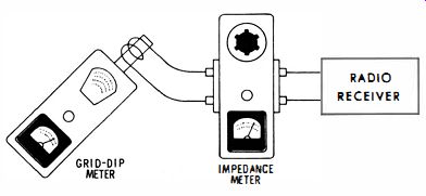
Fig. 6. Checking input impedance of radio receiver.

The RF input impedance of a TV receiver can be checked by means of a skeleton bridge, as shown in Fig. 7 A. In order to minimize the error due to stray capacitances, a compact bridge is made up from three 300-ohm (or other value ) composition resistors. The fourth arm of the bridge consists of the input to the RF tuner. An RF sweep generator is used to drive the bridge. A scope is connected to the looker point on the RF tuner, and the AGC line is clamped. A response curve is displayed on the scope screen, as illustrated in Fig. 7B. The test is made by shorting the diagonal terminals of the bridge as indicated by the dotted line. Then, if the curve does not change in height, the RF input impedance is 300 ohms; but if the curve does change in amplitude, the input impedance is not 300 ohms.

The value of RF input impedance is determined chiefly by the coupling of the input transformer (Fig. 8) . Tighter coupling provides a lower input impedance, and vice versa. The value of input impedance is controlled to some extent by the damping resistance Rl1. Of course, the HF resistance of the coil windings are also a factor. At resonance, inductive and capacitive reactances cancel each other, leaving only the effective resistance of the input circuit.

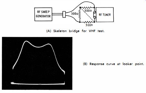
Fig. 7. Checking input impedance of a TV receiver. (A) Skeleton bridge for VHF test. (b) Response curve at looker point.

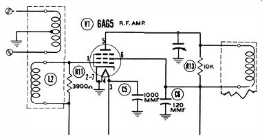
Fig. 8. Coupling controls input impedance.

HIGH-FREQUENCY CAPAC ITANCE TESTS

Capacitors that operate at high frequency must have very little residual inductance. High-frequency operation for an electrolytic capacitor will usually be low-frequency operation for a mica capacitor ; therefore, the consideration is relative.

In a video amplifier you may find an electrolytic bypass capacitor shunted with a comparatively small fixed capacitor, as shown in Fig. 9. At higher video frequencies, the inductive reactance of various electrolytic capacitors becomes excessive and impairs the bypassing action. However, the small fixed capacitor has negligible inductive reactance, and it has a low capacitive reactance at higher video frequencies.

Thus, at 4 mhz, a 5,000-mmf capacitor has about 8 ohms of reactance, while the effective reactance of some electrolytic capacitors at 4 mhz is objectionably large. To demonstrate this fact in a circuit as depicted in Fig. 9, drive the grid of the tube with a signal generator at 4 mhz. Connect a VTVM at the output of the amplifier. Then disconnect C46, and observe the reduction in gain. If C2 has excessive reactance at 4 mhz, you will see the gain go down when C46 is disconnected.

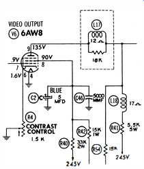
Fig. 9. C46 bypasses inductive reactance.

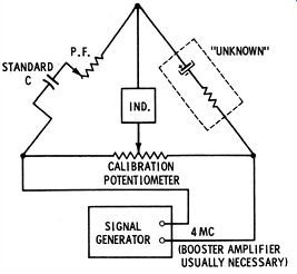
Fig. 10. Test for HF characteristic of electrolytic capacitor.

Bridge Test of Capacitor

To check the frequency dependency of an electrolytic capacitor, use an ordinary capacitance bridge, but drive the bridge at the chosen frequency of test (such as 4 mhz) , as illustrated in Fig. 10. A signal generator is suitable, provided it has a high-level output. Otherwise, a booster amplifier must be used between the generator and the bridge, or a high-level test oscillator employed. In any case, sufficient driving voltage must be applied to the bridge to obtain a useful null-indication. An electrolytic capacitor which tests good at 60 cycles may show a large reduction in capacitance as the driving frequency is increased.

You may find that the null indication is not complete at higher test frequencies; at 4 mhz it might be impossible to obtain even a partial null. Clearly, such an electrolytic capacitor does not even "look like" a capacitor at the test frequency. By varying the bridge-driving frequency, you can find the upper limiting frequency at which the electrolytic capacitor has substantial effective capacitance and a reasonably low power factor. Also, you can calculate the value of the small fixed capacitance that must be shunted across the electrolytic capacitor to obtain good bypassing action over the desired frequency range.

Capacitors With Negative Temperature Coefficient

You will find capacitors in critical circuits such as local oscillator circuits, which have a negative temperature co-efficient. For example, C207 in Fig. 11 is an N220 type. This means that it normally loses 220 parts in 106 of its rated capacitance (2.7 mmf) per degree centigrade. This is too small a variation to check out on a service bridge and many lab-type capacitance bridges are inadequate to check this low value.

Hence, the only practical test is a substitution test. If the local oscillator drifts excessively in frequency and the temperature compensating capacitor is suspected, replace the capacitor, and observe the resulting circuit action.

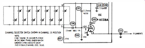
Fig. 11. C207 has negative temperature coefficient.

Distributed Capacitance of H F Coils

The distributed capacitance of high-frequency coils is measured in the same manner as explained in Section 2 for air-core coils in general. Resonant-frequency measurements are made with a grid-dip meter or with equivalent means, with precision fixed capacitors connected across the coil. Then, L/f2 values are plotted against capacitance values, to calculate the distributed capacitance of the coil.

Stray Capacitance of a Circuit

Direct measurement of stray circuit capacitance is usually difficult at high frequencies because the associated circuit resistance complicates the test procedure. Moreover, the circuit resistance is often associated with DC voltage. However, it is quite easy to measure stray capacitance indirectly, in terms of resonant-frequency shift. Consider, for example, the measurement of stray capacitance in the plate circuit of V3, Fig. 12.

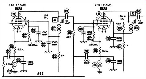
Fig. 12. L17 is reference in measurement of stray capacitance.

This capacitance is different when the tubes are operating. In general, we are interested in the "hot" stray capacitance value.

With the receiver turned on, first measure the resonant frequency of L17 in Fig. 12 with a grid-dip meter. Then, turn the receiver off, and disconnect the leads from L17. Connect a small trimmer capacitor across L17, as depicted in Fig. 13.

Now, adjust the trimmer capacitor to obtain the same resonant frequency as before. Clearly, the trimmer then has the same capacitance as the effective capacitance of the complex RC network in Fig. 12. Then disconnect the trimmer, and measure its value on a capacitance bridge. The reading obtained is the value of the effective circuit capacitance.

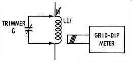
Fig. 13. Capacitor is adjusted for reference resonant frequency.

The coil should not be removed from the receiver in this test, because the proximity of metal surfaces and objects affects its resonant frequency. It is of no concern what this effect may be-the essential point is not to disturb its value.

In addition, use the same separation between the IF coil and grid-dip meter tank in both measurements-if you change the separation, the resonant frequency will be affected, and the measurement will become inaccurate.

Input Capacitance of RF Probe

The input capacitance of an RF or demodulator probe is a figure of merit. The lower is the input capacitance, the better is the probe in signal-tracing applications. It might be supposed that the input capacitance of a HF probe is constant, but this is not so. It varies somewhat with frequency. To measure the input capacitance of a probe at a chosen frequency, select or wind a small coil that is resonant at the frequency of interest when it is shunted by the probe (Fig. 14A). A grid dip meter is used to check the resonant frequency of the coil with the probe shunted across the coil.

(A) Measure the resonant frequency.

CAPACITANCE BRIDGE

(B) Adjust trimmer for same resonance.

(C) Measure value of trimmer capacitor.

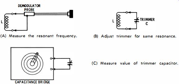
Fig. 14. Measurement of HF probe input capacitance.

Next, disconnect the probe, and connect a small trimmer capacitor across the coil (Fig. 14B). Adjust the trimmer to obtain the same resonant frequency as before, and measure the trimmer capacitance (Fig. 14C ). If the test is repeated at 1, 20, 50, and 100 mhz, for example, somewhat different values of input capacitance will be measured. Note that when semiconductor diodes are employed in the probe under test, it makes no difference whether the probe is connected to a scope or to a VTVM. Conversely, if a vacuum-diode type of RF probe is under test, it must be powered from its associated VTVM. Otherwise, the measurement of input capacitance will be incorrect.

The input capacitance of both semiconductor and vacuum tube HF probes depends to some extent on the signal level that is applied. This variation can be tested by using different separations of the coil (L in Fig. 14) from the grid-dip tank.

Close coupling induces a large voltage in the coil and provides a high-level test ; on the other hand, loose coupling provides a low-level test.

HIGH-FREQUENCY INDUCTANCE TESTS

Shop tests of inductance at high frequencies are seldom concerned with inductance values as such. However, laboratories, factories, and incoming-inspection departments must often measure inductance values at high frequencies. A 1- khz bridge will measure inductances as small as 10 microhenrys.

To measure smaller inductance values, a higher test frequency must be used, so that the small inductance will have appreciable reactance. Various methods are utilized, the simplest of which requires only a grid-dip meter and a pair of precision fixed capacitors.

Grid-Dip Meter Test

The grid-dip meter should have good accuracy and be loosely coupled to the coil under test. The distributed capacitance of the coil is first measured, as previously explained. Here is an example for a small coil : Two fixed capacitors are employed, having values of 10 mmf and 20 mmf, respectively. When the 10-mmf capacitor is shunted across the coil, the grid-dip meter measures a resonant frequency of 18.2 mhz. On the other hand, when the 20-mmf capacitor is shunted across the coil, the resonant frequency measures 14.1 mhz. The corresponding 1/f2 values are 0.003 x 10^-12, and 0.005 x 10^ -12, respectively. Accordingly, the distributed capacitance of the coil is 5 mmf, as shown in Fig. 15.

Inasmuch as the resonant frequency of the coil was 18.2 mhz when shunted by a total of 15 mmf, these values can be substituted in the resonant-frequency formula (f = 1/ (2 pi LC) , from which the inductance is calculated as 5 microhenrys.

The calculation is even simpler from the plot of Fig. 15. The slope of the plotted line is proportional to inductance. When multiplied by 1/ (4 pi^2) the inductance value is obtained. Note that the slope is equal to 0.005 x 10^-12 divided by 20 x 10^-12, or simply 0.005/20, which is 0.0002. Now, 1/ (4 pi^2) is approximately equal to 0.0253, which when multiplied by 0.0002 gives an inductance of 5 microhenrys as before.

Bandwidth and Q

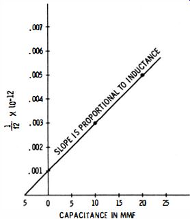
Fig. 15. Distributed cap. is 5 mmf.

If a coil were an ideal inductance, it would have no distributed capacitance and no resistance. Because distributed capacitance is present, the coil has a self-resonant frequency, and because high-frequency resistance is present, the coil has a certain bandwidth. Recall that Q = X,jR ; the Q of the coil is inversely proportional to bandwidth. Generally, the Q and bandwidth of an isolated coil is of minor concern ; the practical consideration is two bandwidth or Q in a particular circuit.

For example, in an IF amplifier the coil is shunted by the dynamic plate resistance of a tube, as depicted in Fig. 16A.

To test the coil for its in-circuit bandwidth, three measurements are made. The signal generator is first tuned for maximum reading on the VTVM ; this determines the resonant frequency, fro Then, the generator is tuned below fr to obtain a VTVM reading that is 70.70;0 of the initial reading. This determines the frequency fl (Fig. 16B) , which is one of the "half-power" frequencies. Next, the generator is tuned above fr to determine the other half-power frequency f2.

The bandwidth is then equal to f2-f1.

The Q-value is given by the formula fr/ (f2-f1 )'

Half-Power Points

The half-power points are called that, because the power in the circuit is equal to E?/R. The VTVM reads E. When the power drops one-half, its value is given by E2/ (2R) . Since the VTVM does not read E? but instead reads E, the half-power point occurs where the VTVM reading is 70.7ro of maximum.

Now, the Q is equal to the resonant frequency divided by the frequency interval between the half-power points. However, the bandwidth is defined by convention, and in the case of communication circuits it is defined as the frequency interval between the half-power points.

(A) Setup for bandwidth and Q measurement. (B) Bandwidth at the half power points.

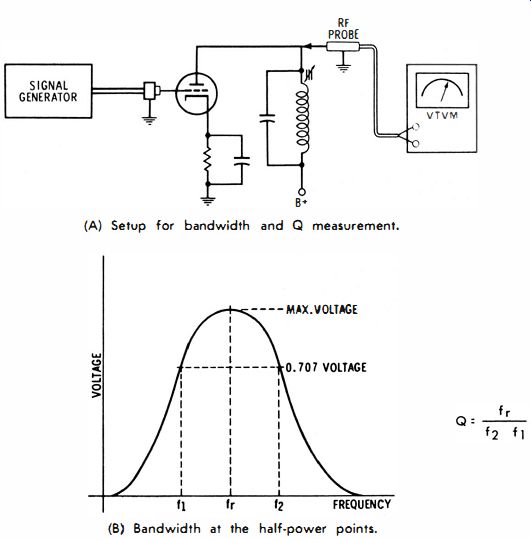
Fig. 16. Measurement of Q and bandwidth.

A different bandwidth is customarily defined in video circuits. In this case, the bandwidth is taken as the frequency interval between the half-voltage points, as illustrated in Fig. 17. Since power is equal to E2/R, the half-voltage points correspond to the 1/4 power points on the curve. Beginners are sometimes confused by the difference in bandwidth definitions for radio and TV receivers. Another source of confusion is the tendency of some apprentices to assume that that bandwidth is given by the frequency interval along the baseline (where the ends of the curve meet the baseline). The foregoing discussion should clarify these considerations.

Coils in Front Ends

The coils in a front end can be checked effectively only by sweep-alignment procedures. Of course, if a coil is shorted or open, the RF signal does not pass, and it can be localized by analysis of receiver operation analysis or by signal-tracing tests. However, the usual problem in the service shop is to adjust the coil inductances to exact values for optimum operation. You will find that coils in front ends may have no slugs or trimmer capacitors. Inductance adjustment is made simply by compressing or expanding the coil turns. This is not difficult, because the coils are wound from soft copper wire, which easily takes a set.

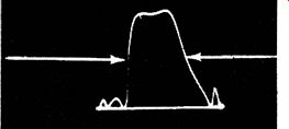
Fig. 17. Bandwidth is measured at half voltage points.

High-band coils may have less than one complete turn. They often have a "hairpin" shape. To adjust their inductance, simply spread the hairpin out wider, or squeeze it closer together. Correct inductance is obtained when the RF response curve matches as closely as possible the shape specified in the receiver service data. RF alignment is exacting and cannot be discussed in detail here. Interested readers are referred to specialized texts, such as Practical TV Tuner Repairs, published by Howard W. Sams.

Detector Diodes

Detector diodes, such as used in video-detector circuits and demodulator probes, operate at comparatively' high frequencies. An ohmmeter test at zero frequency shows only roughly whether a diode is good or bad. Two diodes, both of which check out satisfactorily on an ohmmeter test, might have widely different efficiencies in high-frequency detector application. Laboratories utilize suitable test equipment to test detection efficiency at a chosen frequency. However, in the service shop, the cost of this specialized test equipment cannot be justified-instead, a comparison test is employed and is almost as effective.

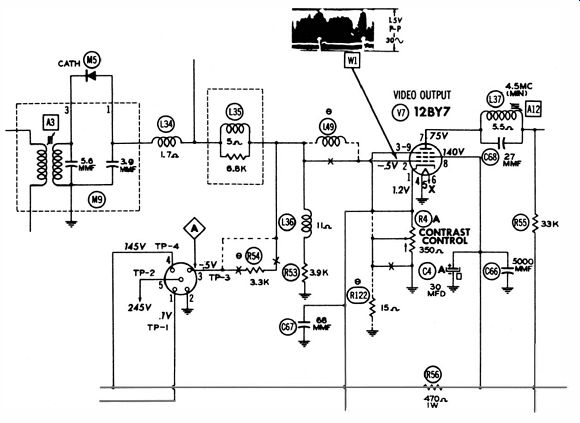
Fig. 18. Typical video-detector circuitry.

A typical video-detector and output configuration is shown in Fig. 18. To make a comparison test of sample diodes, proceed as follows : Connect a scope with a low-capacitance probe to the grid of the video-amplifier tube. Clamp the AGC line. Apply a test signal to the receiver from a pattern generator, or the output from an AM generator can be used. W1 in Fig. 18 shows a typical video-signal pattern. In this test, only the amplitude of the pattern is of interest. When different types of diodes or different diodes of the same type are connected in the M5 circuit, the pattern amplitude will be seen to change. The best detection efficiency, of course, is indicated by maximum pattern height.

Diode in Demodulator Probe

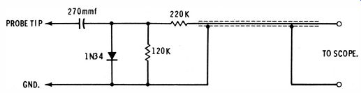
Fig. 19. Schematic of demodulator probe.

The diode in a demodulator probe operates as a simplified video detector. However, the requirements are specialized. The probe is often used in very low-level signal circuit, and so we are chiefly concerned with its small-signal efficiency. A small-signal test can be made as follows : Connect the probe output cable to the vertical-input terminals of a scope. Drive the probe from an IF sweep generator. Advance the scope gain to maximum, and reduce the output from the sweep generator until a pattern about one inch high is displayed on the scope screen.

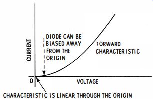
Fig. 20

Now, try substituting different types of diodes, and different diodes of the same type, in place of the IN34 depicted in Fig. 19. The pattern height on the scope screen will change.

The best small-signal efficiency, of course, is indicated by maximum pattern height. Although it is not generally known, the small-signal efficiency of a semiconductor diode can often be improved by a low forward bias. The reason follows:

Improving Detection Efficiency

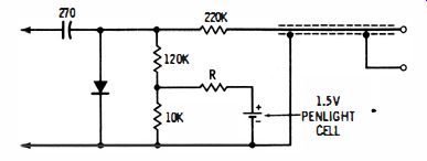
Fig. 21

Recall that a semiconductor diode is a nonlinear resistance.

Best detection efficiency is obtained when the characteristic curve changes most rapidly. Now, all semiconductor diodes have a practically linear characteristic through the origin, as depicted in Fig. 20. In other words, at extremely small signal levels, the detection action is practically zero. However, as the operating point is moved into the forward-current region of the diode, the characteristic is no longer linear but starts curving upward. Hence, if the diode is biased a fraction of a volt into the forward-current region, the small-signal detection efficiency improves considerably, at least for most commercial diode types.

You can add a penlight cell in a voltage-divider circuit to a demodulator probe, as shown in Fig. 21, and usually obtain improved small-signal sensitivity. The value of R can only be determined by experiment-it varies for different diodes. Choose the value that provides maximum pattern height on the scope screen.