Basic Waveform Characteristics [Scope Waveform Analysis (1963)]

Waveforms are characterized not only by shape, frequency or frequencies, and rise time, but also by voltage and phase.

The amplitude of a waveform is always of importance in test work; it is sometimes more significant than waveshape. Amplitude means the largest excursion of the wave, measured in peak-to-peak volts, amperes, or milliamperes. Since the scope can measure the voltage drop across a known value of resistance, the amplitudes of either voltage or current waveforms can be measured with a scope.

Scope patterns indicate the peak and the peak-to-peak voltages of a waveform if the scope is suitably calibrated. The relations of these voltages in a sine wave are depicted in Fig. 3-1A. Note that in a sine wave the positive-peak voltage is equal to the negative-peak voltage, the peak-to-peak voltage is equal to twice the peak voltage, and the root-mean-square (rms) voltage is equal to 0.707 of the peak voltage.

You will find that the positive-peak voltage in a complex waveform is generally different from the negative-peak voltage.

This fact is illustrated in Fig. 3-1B. When no input voltage is applied to the scope, the trace rests at a certain reference level on the screen. This is the zero-volt level. When a complex waveform voltage is applied to the scope input terminals, the waveform is displayed in a certain relation to the reference (zero volt) line, as seen in Fig. 3-1B.

(A) Sine wave. (B) Unsymmetrical waveform.

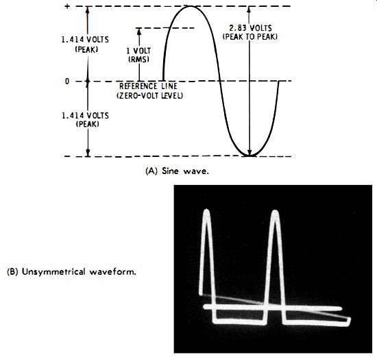
Fig. 3-1 . Peak voltage relations.

The zero-volt line divides the complex waveform into a positive half cycle and a negative half cycle. The excursion above the zero-volt line gives the negative-peak voltage. The total excursion (sum of positive- and negative-peak voltages) gives the peak-to-peak voltage of the waveform.

The positive-peak voltage is not necessarily equal to the negative-peak voltage in a complex waveform, but the area of the positive half cycle is always equal to the area of the negative half cycle. This results from the fact that there is just as much positive electricity as negative electricity in each cycle. Horizontal deflection is linear in time when sawtooth deflection is used, and electrical quantity is given by the product of voltage and time.

Otherwise stated, the positive and negative excursions of the Fig. 3-1 waveforms enclose exactly equal areas. You would judge this to be true by simple inspection. If you have a knowledge of calculus, you can integrate voltage with respect to time for a generalized complex waveform and prove this fact analytically. The scope is operating as an electronic computer in this application; it automatically performs the integrations and separates the equal areas at the zero-volt level. This is an analog-computer situation.

PEAK-TO-PEAK, RMS, AND DC VALUES

The rms voltage is 0.707 of the peak voltage only for a sine wave. Any complex waveform has a different rms value. The rms voltage of a complex waveform cannot be measured directly with a scope or with ordinary service voltmeters. What is the significance of an rms voltage ? This concerns the power developed by a waveform. For example, if a soldering iron is heated from a 117-volt rms AC line, it will develop just as much heat as when powered from a 117 -volt DC line. In other words, the rms voltage of a waveform relates it to a DC voltage that will produce the same amount of power in a resistor. In most situations you are concerned only with the power developed by a sine wave; hence, the rms voltages of complex waveforms are not of general interest.

Peak-to-peak voltages are of chief concern in analysis of waveforms generated by electronic circuitry. In certain situations a peak voltage is also significant. There is an important relation between peak-to-peak and DC voltage values which is encountered in working with DC scopes. Recall that a DC scope can be calibrated either from a sine-wave or a DC voltage source, as mentioned in the preceding Section. This fact results from the equal deflections produced by a given value of either DC or peak-to-peak AC voltage. If you apply + 10 volts to the vertical input terminals of a DC scope, the beam will be deflected upward by a certain amount; if you apply -10 volts, the beam will be deflected downward by the same amount. If you apply a 10-volt peak-to-peak AC input to the scope, the excursion of the beam will be the same as if 10 volts DC were applied. To put it another way, it makes no difference whether the DC scope is calibrated from a 10-volt DC source or a 10 volt peak-to-peak AC source. In either case you will step off the same number of vertical intervals.

Note that if you apply a DC input voltage to an AC scope, the beam merely flicks up (or down, depending on polarity) and promptly comes to rest at its original level. The reason for this transient action is that an AC scope utilizes an RC-coupled vertical amplifier. The coupling capacitors will not pass DC, because a DC voltage has zero frequency, and a capacitor has infinite reactance at zero frequency. Inasmuch as DC cannot be passed, why does the beam nevertheless flick up momentarily when you apply a DC voltage? This happens because the sudden application of the DC voltage is equivalent to the leading edge of a square wave. Thus, the scope responds just as if a square-wave voltage had been applied.

If you apply a DC voltage to the vertical input terminals of an AC scope then break the connection and apply the voltage once again, the beam does not respond the second time. This is because the first application charged up the input coupling capacitor, and the capacitor (if good) holds this charge. Of course, if the capacitor is leaky, the beam will flick on the second application of the DC voltage. Hence, this is a quick check which shows whether the input coupling capacitor to the AC scope is defective and may need replacement. Eventually, of course, any charged capacitor will discharge itself, because insulation resistance is never infinite. Nevertheless, the input coupling capacitor in an AC scope should hold a charge for at least 5 or 10 seconds.

RESISTANCE WAVEFORMS

Everyone is familiar with the use of an ohmmeter to measure resistance. A scope can also be used to measure resistance. It has the advantage of high sensitivity with fast response to change in resistance. A common example of a resistance waveform is the output from a strain gauge. Wire changes its resistance when it is strained in extension or compression. Hence, if a zig-zag length of wire is bonded to an insulating sheet and cemented to some structure (such as a girder) which is subjected to varying forces, the resistance of the wire (strain gauge) changes with any bending of the structure.

If a constant current is passed through the strain gauge, and the vertical input leads of a scope are connected across the gauge terminals, the scope deflection will be proportional to resistance. The resistance variation which produces the scope waveform may be rapid or slow; it is always in step with the varying forces applied to the structure under test. If the resistance waveform has a slow variation, a DC scope is used.

Resistance waveforms with rapid variation can be displayed accurately on an AC scope.

Thus, simple test setups suffice to display the three basic electrical parameters of voltage , current, and resistance. While voltage waveforms are most commonly utilized, current waveforms are often of interest also. Resistance waveforms are less common, although they are quite familiar to technicians in various branches of industrial electronics.

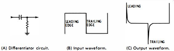
Fig. 3-2. Differentiator action. (A) Differentiator circuit. (B) Input waveform. (C) Output waveform.

PRINCIPLES OF DIFFERENTIATION

Fundamentals of differentiation were mentioned in the preceding Section. Basic principles of the differentiating action will now be explained. If a differentiating circuit has a short time constant and a square wave is applied, the peak-to-peak output voltage is twice as great as the input voltage, as indicated in Fig. 3-2. The initial spike or surge has the same peak-to-peak voltage as the square wave, and it soon decays practically to zero. The second spike or surge is in the opposite polarity and also has the same peak-to-peak voltage as the square wave. Hence, the peak-to-peak amplitude of the output waveform in this case is double the amplitude of the input square wave.

What about the harmonics in the differentiating output? First, you will find the same harmonic frequencies present as in the square wave itself. However, the differentiating circuit weakens the low frequencies with respect to the high frequencies. Hence the relative voltages of harmonics in the differentiated output are not the same as in the input square wave.

Harmonic Amplitudes in a Differentiated Square Wave

Recall that a square wave consists of a fundamental frequency plus many odd harmonics of this fundamental frequency. When a square wave is passed through a differentiating circuit, each of its frequencies can be considered apart from all of the other frequencies. That is, you can consider the circuit action with respect to the fundamental by itself, with respect to the third harmonic by itself, and so on. Then, if you add up all the separate outputs, you will obtain the differentiated waveform.

Suppose that a differentiating circuit contains a 2700-mmf capacitor and a 1-megohm resistor. If you apply a 60-cycle square wave to the circuit, the fundamental frequency is 60 cycles. The capacitor has a reactance of about 1 megohm at 60 cycles. Hence, the fundamental is attenuated to 71% of the input level by passage through the differentiating circuit. Next, the third harmonic in the square wave has a frequency of 180 cycles. The capacitor has a reactance of about 330,000 ohms at this frequency. Hence, the third harmonic is attenuated to 94% of its input level by passage through the differentiating circuit.

The fifth harmonic has a frequency of 300 cycles, and the capacitor has a reactance of 200,000 ohms at this frequency; therefore, the fifth harmonic is attenuated at 98% of its input level by passage through the differentiating circuit.

How then does it happen that although the differentiating circuit weakens all the harmonics and weakens the low- frequency voltages more than the high-frequency voltages, the end result is a waveform with twice the original amplitude? The reason is simply that the harmonics are also shifted in phase by the differentiating circuit. This phase shift is such that the peaks of all the harmonics are moved closer together during the pulse than in a square wave. As a result, the sum of the harmonic voltages at the instant of peak voltage is greater than before their phases were shifted.

BASICS OF RC CIRCUIT ANALYSIS

The foregoing review of harmonic amplitudes in a differentiated square wave gives a general picture of differentiating circuit action. Now, it will be helpful to explain the basics of the analysis. First, it was stated that the reactance of a 2,700 mmf capacitor is about 1 megohm at 60 cycles. How do you know this? You can read the answer from a reactance slide rule, or you can calculate the reactance from the relation:

1 Xc = 2 pi fC

where, Xc is the capacitive reactance in ohms, Pi is 3.1416, f is the frequency in cycles per second, C is the capacitance in farads.

When the arithmetic is performed, the answer is found to be about 1 megohm.

Next, it was stated that the fundamental is attenuated to 71% in passing through the differentiating circuit. How do you know this? The attenuation is seen from the triangle shown in Fig. 3-3B. The triangle shows the ohms relation in an RC circuit.

To remind yourself that reactive ohms add at right angles to resistive ohms, you may find it helpful to draw reactive ohms with a different symbol than resistive ohms. The input voltage is applied across the impedance, which has a value of 1.414 megohms. You do not need to make the calculation-simply scale off the impedance with a ruler. Inasmuch as the I-megohm resistance is approximately 71% of the 1.414-megohm impedance, it follows that the voltage across the 1-megohm resistor is attenuated to 71% of the input voltage.

It is apparent from the diagram in Fig. 3-3A that a differentiating circuit acts simply as a voltage divider. The only complication is that since it is an AC voltage divider, the two different types of ohms must be combined at right angles. The RC circuit is almost, but not quite, as easy to work out as an ordinary resistive voltage divider. It is quite essential that you see the difference between DC and AC circuit response, because all waveforms are based on AC circuit response.

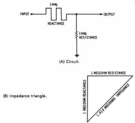
Fig. 3-3. Impedance relationship in an RC circuit. (A) Circuit. (B) Impedance triangle.

The circuit response to the third harmonic is determined in the same way as has been described for the fundamental. The only difference is that the third harmonic has three times as high a frequency as the fundamental so that the capacitive reactance is only 1/3 as great, or 330,000 ohms. In turn, the ohms triangle has different proportions, and the third harmonic is attenuated to 94% by the differentiating circuit. It is by no means implied that you will need to make this graphical analysis when you are called on to analyze differentiating action in a circuit. On the other hand, it is vital that you understand why the circuit weakens the low frequencies with respect to the high frequencies.

Understanding Phase Shift

The maximum phase shift that can be theoretically obtained in a differentiating circuit is 90°. The reason for this limit is that the current leads the voltage by 90° in a pure capacitance.

In a differentiating circuit the current into the capacitor causes a voltage drop across the circuit resistance. Inasmuch as voltage and current are in phase in a resistance, the voltage output from a differentiating circuit has the same phase as the current. If the capacitive reactance is very large compared with the resistance in the circuit, the output voltage will be shifted almost 90° in phase. On the other hand, if the capacitive reactance is very small, the output voltage will have practically the same phase as the input voltage.

Beginners occasionally have difficulty in understanding why current and voltage are 90° out of phase in a capacitor. Understanding of this relation is easy when the capacitor is recognized as an electrical storage device. A capacitor can be compared with a tank of compressed air-the more air pressure you apply to the tank, the more air you force into the tank. Similarly, if you apply more voltage to a capacitor, you will force more electrical charge into the capacitor. The capacitor exerts an opposition to the incoming current, just as a tank of compressed air exerts a back pressure against the air that you are forcing into it.

If you open a valve in a tank of compressed air, the air flows out; similarly, if you connect a wire across a charged capacitor, its electric charge flows out. If you increase the voltage across a capacitor, electricity is being stored in the capacitor as long as the voltage is increasing; if you decrease the voltage across a capacitor, the stored energy flows out of the capacitor. If you increase the voltage across a capacitor quickly, electricity flows into the capacitor quickly; if you increase the voltage across a capacitor slowly, electricity flows into the capacitor slowly.

Common-Sense Analysis

Suppose you decrease the voltage across the capacitor quickly-the stored charge then flows out quickly. But if you decrease the voltage across the capacitor slowly, the stored charge flows out slowly. These basic facts are obvious. Now refer to Fig. 3-4. As the voltage E starts to rise from zero, it increases rapidly. Hence, current flow into the capacitor is rapid.

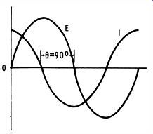
Fig. 3-4. Phase relationship in pure capacitance.

On the other hand, as E approaches the 90 ° point, the voltage levels off and ceases to increase at its peak. In turn, no more current flows into the capacitor at the peak-voltage point-the current flow has dropped to zero at this point. This is the same as saying that the current flow is zero when the voltage is maximum. The same common-sense analysis can be applied to the interval from 90° to 180°, during which time current is flowing out of the capacitor. To summarize, it is clear that the current flow must be 90° out of phase with the voltage across a capacitor.

Resistance and Capacitance in Series

It is interesting to consider the phase relation between current and voltage when capacitance and resistance are connected in series (as in a differentiating or integrating circuit) . Fig. 3-5 shows this situation. If you take the output from across the resistor, the circuit is called a differentiating circuit; if you take the output from across the capacitor, it is called an integrating circuit. In either case the phase difference between the input voltage and the current is obviously the same. Again, a sine-wave voltage is applied to the circuit for a common-sense analysis of phase.

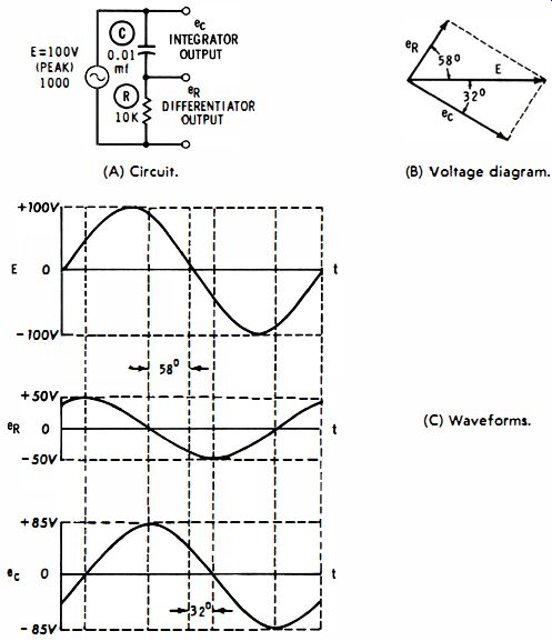
Fig. 3-5. RC circuit relationships. (A) Circuit. (B) Voltage diagram. (C) Waveforms.

The same general principle previously explained for a pure capacitance applies in this case. Current flows into the capacitor when the voltage is increased; conversely, current flows out of the capacitor when the voltage is decreased. If the voltage is increasing rapidly, the current flow increases rapidly, and vice versa. However, there is a difference in circuit action caused by the series resistance. The resistance slows down the rate at which the capacitor can be charged or discharged.

This simply means that the current flow tends to lag behind the voltage. To put it another way, voltage E is increasing most rapidly as it rises from zero, but the peak current flow is now delayed somewhat due to the opposition of the resistance. For the values given in Fig. 3-5, the peak of current flow does not occur until 32 deg after the voltage starts its rapid rise. Likewise, current flow does not fall to zero until 32 deg after the voltage has passed its peak and is no longer increasing. The resistance reduces the rate of outflow of current from the capacitor, just as it reduces the rate of inflow of current into the capacitor.

Phases in RC Series Circuits

As just explained, current flow does not lead the voltage by 90° in an RC series circuit. Instead, the current flow leads by less than 90 degr. For the particular values used in Fig. 3-5, the current lead is 58°. It is evident that if you choose a very large value of resistance, the current lead will become very small and approach 0° as a limit. From another point of view the reactance of the capacitor becomes negligible when you make the resistance extremely large-effectively, the circuit tends to look like a pure resistance to the source voltage.

On the other hand, when you make the series resistance extremely small, its value becomes negligible with respect to the reactance of the capacitor. If the resistance is so small that it can be practically disregarded, the circuit looks like a pure capacitance to the voltage source. Thus, the output voltage from the circuit can be made to differ in phase from the input voltage over the range from practically zero to 90°. This is the fundamental principle of simple phase-shifting circuits which are widely used in both service and industrial equipment.

Phase Shift With Square Wave Applied

With these simple facts in mind it is easy to see why the various harmonics are shifted in phase by different amounts when a square wave is applied to an RC series circuit. Each harmonic has a different frequency, which means that the capacitor has a different reactance for each harmonic. Returning to the former example of a 2700-mmf capacitor connected in series with a 1-megohm resistor, recall that the capacitor has a reactance of about 1 megohm at 60 'cycles, a reactance of 0.33 megohm at 180 cycles, and a reactance of 0.2 megohm at 300 cycles. The phase angle between output and input is large when the frequency is low (60 cycles) ; but the phase angle between output and input is small when the frequency is high (300 cycles) . Knowing that low frequencies will be shifted in phase more than high frequencies by a differentiating circuit, you are now in a good position to recognize that the peaks of the harmonics in a square wave are all shifted by the circuit action, as is evident from Fig. 3-6. In both of the diagrams the fundamental is taken as the reference. Consider the effect of differentiation on the phase of the third harmonic. In the square wave (Fig. 3-6A) the third harmonic has a negative peak which subtracts from the positive peak of the fundamental, thereby making the resultant waveform flatter than a sine wave. On the other hand, in the pulse (Fig. 3-6B) , the third harmonic has a positive peak which adds to the positive peak of the fundamental, thereby making the resultant waveform more pointed than a sine wave.

A: FUNDAMENTAL B: 3D HARMONIC C: FUNDAMENTAL PLUS 3D HARMONIC

D: 5TH HARMONIC, E: FUNDAMENTAL PWS 3D AND 5TH HARMONICS, F: 7TH HARMONIC G: FUNDAMENTAL PWS 3 D. 5TH, AND 7TH HARMONICS

A FUNDAMENTAL B 3RD HARMONIC C FUNDAMENTAL PWS 3RD HARMONIC (A) Square wave. (B) Pulse.

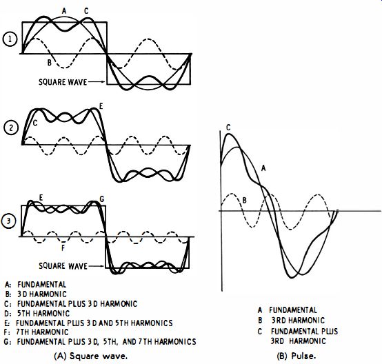
Fig. 3-6. Harmonic phase relationships.

You can form a pulse from the same harmonics as are present in a square wave. To do so, you need merely shift the phase of each harmonic so that all positive peaks occur at the same instant. A differentiating circuit has this general action. To see why this is so, first observe the relative harmonic phases in the square wave (Fig. 3-6A) . Note that all harmonics start in phase with the fundamental of a square wave. In other words, each harmonic starts rising from zero voltage at the start of the square wave.

This is no longer the case after the square wave has passed through a typical differentiating circuit; the fundamental is shifted 45 ° from its original position, the third harmonic is shifted 18° from its original position, and the fifth harmonic is shifted 11 ° from its original position. What this means with regard to the peaks of the waveforms is shown in Fig. 3-6. In the square wave the fundamental and the third harmonic have opposing positive and negative peaks. On the other hand, in the differentiated wave the fundamental and third harmonic have essentially aiding peaks. If you plot the shift of the fifth harmonic, you will see that it too will aid the fundamental peak in the differentiated wave.

Sharpness of Differentiated Wave

As you know, the output from a differentiating circuit with a very short time constant is a sharp spike. On the other hand, the output from a differentiating circuit with a long time constant is a much broader pulse. In terms of harmonic phase shift, the short time constant brings the peaks of the harmonics into a highly aiding position, but a long time constant brings the peaks of the harmonics into only a partially aiding position.

It is not anticipated that you will need to go through this analytical procedure when you are evaluating the action of a differentiating circuit. However, it is important to understand what is happening in the circuit from a qualitative standpoint.

Unless you recognize the circuit actions which underlie waveforms, you will be baffled and fail in attempts to analyze practical situations. If you understand why a certain type of waveform appears on the scope screen, you are then in a position to recognize the circuit action behind the waveform. This circuit action may be normal or abnormal, depending on the particular circumstances. If the waveform is abnormal, your ability to analyze the pattern will guide you to the circuit defect that is causing the abnormal waveform.

KIRCHOFF'S LAW

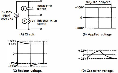
Fig. 3-7. RC differentiator and integrator action on a square wave. (A) Circuit. (B) Applied voltage. (C) Resistor voltage. (D) Capacitor voltage.

Kirchhoff's law applies to all circuits. This law states that the sum of all the voltages around a complete circuit is zero.

Observe how this applies to Fig. 3-7. The generator applies 100 peak volts to the 0.1-mfd capacitor and 10-K resistor in series.

Since a negative charge of 25 volts remains on the capacitor from the preceding cycle, the total voltage across the resistor at the start of the positive half cycle is 125 volts. The sum of the capacitor and resistor drops is 100 volts. This 100 volts opposes the 100 volts of the generator, and the sum of the voltages around the circuit is equal to zero.

Going from peak voltages to instantaneous values, you will find that at every instant the sum of the voltages around the circuit is equal to zero. This is the consequence of the basic characteristics which were shown in Fig. 2-9; Curve B is simply curve A turned upside down. It is an illustrative statement of Kirchhoff's law.

If it seems strange that the voltage drop across the resistor is 25 volts greater than the source voltage, refer to Fig. 3-2. This situation illustrates a short time constant in which the output peak-to-peak voltage is actually twice as great as the input peak-to-peak voltage. Note in Fig. 3-7 that the output voltage decays 25 volts between the leading and trailing edges. The input leading edge still changes 200 volts every time. Hence, the output voltage consists of the difference between the input voltage and the decay voltage. For the example shown in Fig. 3-7, this circuit action makes the peak output voltage 25 volts greater than the peak input voltage.

VOLTAGE AND CURRENT WAVEFORMS

From the previous development it is clear that a waveform may depict either voltage or current. In Fig. 3-7 the integrator output is a voltage waveform; the scope displays the voltage across the capacitor. On the other hand, the differentiator output is a current waveform; the scope displays the current through the resistor. Of course, the scope senses the voltage drop across the resistor while it is displaying the charging current flow into the capacitor.

How is the current measured? Let us suppose that the scope is calibrated for 25 peak-to-peak volts per vertical interval. The differentia tor output is taken across a 10-K resistor. By Ohm's law, the scope calibration then becomes 2.5 milliamperes peak-to-peak per vertical interval. If the differentiator output deflects the beam 10 squares, the peak-to-peak charging current is 25 milliamperes.

DIFFERENTIATION AND INTEGRATION OF SINE WAVES

It is sometimes stated that a sine wave cannot be differentiated or integrated. This is true insofar as waveshape is concerned-the output waveform is always the same as the input waveform. Nevertheless, this assertion neglects considerations of phase. If a sine wave flows in a differentiating circuit, the output voltage leads the source voltage. Or, if a sine wave flows in an integrating circuit, the output voltage lags the source voltage.

These facts follow from the principles which have been noted previously-a capacitor draws a leading current with respect to the source voltage. The output in a differentiating circuit is taken across the resistance; hence, the output voltage is proportional to current flow and leads the source voltage. This fact sometimes causes confusion for the beginner, because he often will ask: "How can a current exist in the circuit before voltage is applied?" This question confuses the steady state which is assumed for sine-wave drive, as contrasted with the transient state which exists for a brief period after the voltage is first applied. This interesting point will be discussed later in this Section.

Now, however, to continue with the sine-wave relations in an RC circuit, the integration of a sine wave results in an output voltage which lags the source voltage. This fact is easily understood by returning to Fig. 3-5, the full implications of which might have escaped you the first time around. When you combine the resistive and reactive ohms in the circuit, each side of the impedance triangle which you draw indicates the phase of its associated voltage. These lines are shown in Fig. 3-5B as arrows all starting from the origin, so that the phase relations are clearly apparent. Here, the voltage across the resistor (en) , is leading the source voltage (E) by 58 degrees. The voltage across the capacitor (ec) is lagging the source voltage (E) by 32°. Inasmuch as these phase relations are established by the resistive and reactive ohms which are present in this circuit configuration, it is clear that the output voltage from an integrating circuit must lag the source voltage by an amount determined by the circuit design.

TRANSIENT AND STEADY STATES OF SINE WAVES

A distinction must usually be made between the transient and the steady state. That is, if you switch a sine-wave voltage suddenly into an RC circuit, the steady-state conditions do not exist at the instant that current starts to flow. But the voltages soon settle down to their steady-state relationships. How long is the transient interval? This depends on the time constant of the circuit. If the time constant is long, it takes more time for the circuit to reach equilibrium with the resistor voltage leading the capacitor voltage by 90°. A specific situation is depicted in Fig. 3-8. Let the voltage across the capacitor be called ec.

Then, by application of Kirchhoff's law (which is not carried out here but may be consulted in textbooks):

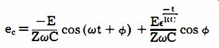
where,

-t

-E Et:HC ec = ZwC cos (wt + cf» + ZwC cos cf) E is the peak applied voltage,

w is 2 pi times the frequency in cycles per second, Z is the circuit impedance, cf> is the angle whose cotangent is wRC, R is the resistance in ohms, C is the capacitance in farads, t: is 2.718.

In the expression for ee, the first term is the steady-state voltage, while the second term is the transient voltage. Eventually, of course, the transient term decays to zero, leaving only the steady-state term. When the switch is first closed, the two terms subtract from each other, because one is positive and the other is negative.

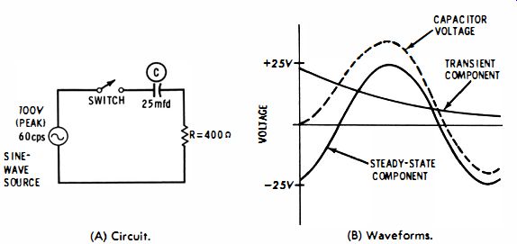
Fig. 3-8. Transient response of series RC circuit. (A) Circuit. (B) Waveforms.

The graph of this equation for the circuit values in Fig. 3-8A is shown in Fig. 3-8B. (The values were chosen to make the transient voltage easily recognizable.) Note that the resultant voltage waveform is the algebraic sum of the steady-state and transient components.

It can be seen from a close study of the equation that the relation between the steady-state and transient components in any given case depends on the values of R and C. In this illustration it was assumed that the switch was closed at the start of the cycle of the applied voltage. If the switch is closed at any other time, the resultant waveform is further altered.

ELIMINATION OF THE TRANSIENT INTERVAL

It is clear that the current cannot lead the voltage at the instant of switching in the foregoing example, because there is as yet no current established in the circuit to lead the voltage. Hence, it might be supposed impossible to devise a switching circuit which could establish the steady state instantaneously.

However, this supposition would be false. Consider an electronic switch which can be set to close at any point you choose along the source waveform. Then, a setting will be found which will establish the steady state instantaneously, with no distortion at all from a transient interval.

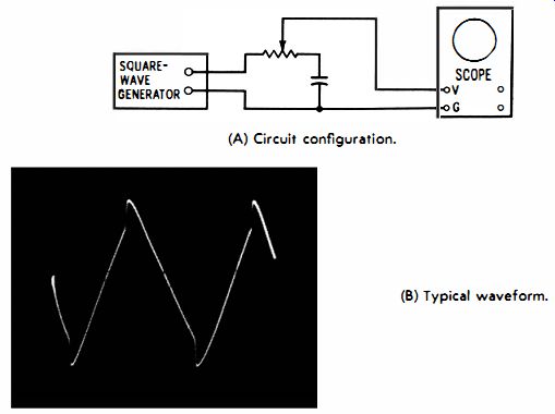
Fig. 3-9. Combined integrator and differentiator. (A) Circuit configuration. (B) Typical waveform.

What is this critical instant for switching which eliminates the transient and establishes the steady state at the outset? This instant corresponds to the phase of the source for which the capacitor voltage will be zero in the steady state. In other words, switching must occur at a phase which normally exists for zero stored energy in the capacitor. The critical phase, in turn, is determined by the time-constant of the RC circuit. At the critical instant, the source voltage is somewhere between its zero and peak values.

Just as it is possible to time an electronic switch so that an AC voltage can be introduced into an RC circuit without transient distortion, it is also possible to time the switch so that the AC voltage can be turned on without distortion in an RL circuit. Of course the timing must be different in this case.

COMBINED DIFFERENTIATION AND INTEGRATION

Some circuits, such as in Fig. 3-9A, operate as simultaneous differentiators and integrators. The output waveform is taken across the capacitor and part of the resistor. The combination waveform can have a wide variety of shapes, depending on how much of the differentiated voltage is introduced, and also on the time-constant of the circuit. A typical output waveform is shown in Fig. 3-9B.