AMAZON multi-meters discounts AMAZON oscilloscope discounts
If you are a novice in the electrical or electronics fields, you will soon discover that this section is not light reading. I'm not suggesting that it will be difficult to under stand, but we are providing an advanced warning that it will be concentrated. This section was designed to maximize reading efficiency. Therefore, there are some basic terms used in conjunction with component descriptions that you might be a little confused about. Don't panic! All unexplained terms are covered later in the section as it becomes more appropriate to do so.
Much forethought has gone into the structure of this and successive sections, in order to provide you with the easiest possible way of comprehending the fundamentals of the electrical and electronics fields. It is not always prudent to define every detail of a topic under discussion because the most important aspects might be obscured by issues that could be more clearly explained in a different context. Therefore, we suggest that you read this section twice. You will find the confusing terms, of the first reading, to be much easier to understand during the second reading. If, after the second reading, you are still a little shaky in a few areas, don't become frustrated. The basics explained in this section will be utilized throughout the guide. We have tried to be thorough in placing reminders throughout the text as an additional aid to understanding.
Also, because we all learn by doing, these same fundamentals will be used in the construction of many practical circuits. In this way, concepts are removed from the realm of theory and put into actual practice. One last suggestion-remember, this is a textbook. Textbooks are not designed or intended to be read in the same way as a good novel; they are designed to be studied. You might have to go back and reread many sections as your progress continues.
Electronic Components
The purpose of this section is to provide the reader with a basic concept of the physical structure of individual electronic components, and how to determine their values.
Resistors
A resistor, as the name implies, resists (or opposes) current flow. As you will soon discover, the characteristic of opposing current flow can be used for many purposes. Hence, resistors are the most common discrete components found in electronic equipment (the term discrete is used in electronics to mean nonintegrated, or standing alone).
Resistors can be divided into two broad categories: fixed and adjustable. Fixed resistors are by far the most common. Adjustable resistors are called potentiometers or rheostats.
Most fixed resistors are of carbon composition. They utilize the poor conductivity characteristic of carbon to provide resistance. Other types of commonly manufactured resistors are carbon film, metal film, molded composition, thick film, and vitreous enamel. These different types possess various advantages, or disadvantages, relating to such parameters as temperature stability, tolerance, power dissipation, noise characteristics, and cost.
The two most critical resistor parameters are value (measured in ohms) and power (measured in watts). Resistors that are larger in physical size can dissipate (handle) more power than can smaller resistors. If a resistor becomes too hot, it can change value or burn up. Consequently, it is very important to use a resistor with adequate power-handling capability, as determined by the circuit in which it is placed. Unfortunately, there is not a good, standard way of looking at most resistors and determining their power rating by some standardized mark or code. Comparative size can be deceiving depending on the resistor construction. For example, a 10-watt wire-wound resistor might be about the same size as a 2-watt carbon composition resistor. Common power ratings of the vast majority of resistors are 1/8, 1/4, 1/2, 1, and 2 watts. Don't worry about being able to determine resistor power ratings at this point. It is largely an experience-oriented talent that you will acquire in time.
The value of most resistors is identified by a series of colored bands that encircle the body of the resistor. Each color represents a number, a multiplier, or a tolerance value. The first digit will always be the colored band closest to one end.
There are two color-coded systems in common use today: the four band system and the five-band system. In the four-band system, the first band represents the first digit of the resistance value, the second band is the second digit, the third band is the multiplier, and the fourth band is the tolerance (resistors with a tolerance of 20% will not have a fourth band). The five-band system is the same as the four-band one, except for the addition of a third band representing a third significant digit. The five-band system is often used for precision resistors requiring the third digit for a higher level of accuracy. There are also a few additional colors used for tolerance identification in the five-band system.
You will need to memorize the following color-code table:
Resistor Color Codes
Black _ 0 Green _ 5
Brown _ 1 Blue _ 6
Red _ 2 Violet _ 7
Orange _ 3Gray _ 8
Yellow _ 4 White _ 9
Brown _ 1% tolerance Yellow _ 4% tolerance
Red _ 2% tolerance Silver _ 10% tolerance
Orange _ 3% tolerance Gold _ 5% tolerance
The following are a few examples of how these color-code systems work. As stated previously, the color band closest to one end of the resistor body is the first digit. Suppose that you had a resistor marked blue gray-orange-gold. Because there are only four bands, you know it uses the four-band system. Therefore:
Blue _ 6 gray _ 8 orange _ 3 gold _ 5% tolerance
The first two digits of the resistor value are defined by the first two bands. Therefore, the two most significant digits will be 68. The third band (multiplier band) indicates how many zeros will be added to the first two digits; in this case it's 3. So, the full value of the resistor is 68,000 ohms. The tolerance band describes how far the actual value can vary. A 5% tolerance means that this resistor can vary as much as 5% more, or 5% less, than the value indicated by the color bands. 5% of 68,000 is 3400. Therefore, the actual value of this resistor might be as high as 71,400 ohms, or as low as 64,600 ohms.
Another example of the four-band system could be red-violet-brown silver. Therefore:
Red _ 2 violet _ 7 brown _ 1 silver _ 10% tolerance
The value of this resistor is 27 with 1 zero added to the end; or 270 ohms. The 10% tolerance indicates it can vary either way by as much as 27 ohms.
Try an example of the five-band system: brown-black-green-brown red. The first three bands are the first three digits: brown-black-green _ 105. The fourth brown band indicates that 1 zero should be added to the end of the first three digits resulting in 1050 ohms. The fifth band is tolerance; red _ 2%.
Just to make things a little more confusing, some manufacturers add a temperature coefficient band to the four-band system resulting in a resistor appearing to be coded in the five-band system. The easy way to recognize this is the fourth band will always be either gold or silver. If this is the case, simply disregard the fifth band. Also, as stated previously, a complete absence of a fourth band indicates a 20% tolerance.
On some precision resistors or larger power resistors, the actual value and tolerance rating might be printed on the resistor body. A variety of typical resistors is illustrated in Fig. 1.
A good way to become very proficient at reading resistor color codes and estimating power ratings (an extremely handy talent to have) is to order one of the large grab-bag resistor specials from one of the mail order surplus stores listed in Section B. Use your DVM (set to measure ohms) to verify that your color-code interpretations are correct. (Don't hold onto the DVM test lead ends with both hands when measuring;
the DVM will include your body resistance in the reading.) You'll wind up with a good assortment of cheap sorted resistors. The experience gained in using your DVM will be a side benefit!
Potentiometers, Rheostats, and Resistive Devices
Technically speaking, a potentiometer is a three-lead continuously variable resistive device. In contrast, a rheostat is a two-lead continuously variable resistor. Unfortunately, these two terms are often confused with each other, even by many professionals in the field.
A few good examples of potentiometers can be found in the typical consumer electronic products around the home. Controls labeled as "volume," "level," "balance," "bass," "treble," and "loudness" are almost always potentiometers.
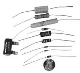
Fig. 1 A sampling of typical resistor shapes and styles.
A potentiometer has a round body, about 1/2 to 1 inch in diameter, a rotating shaft extending from the body, and three terminals (or leads) for circuit connection. It consists of a fixed resistor, connected to the two outside terminals, and a wiper connected to the center terminal. The wiper is mechanically connected to the rotating shaft, and can be moved to any point along the fixed resistance by rotating the shaft. A rheostat can be made from a potentiometer by connecting either out side terminal to the wiper terminal.
Potentiometers are specified according to their power rating, fixed resistance value, taper, and mechanical design. The fixed resistance value is usually indicated somewhere on the potentiometer body (it can be determined by measuring the resistance value between the two outside terminals with a DVM). If the power rating is not marked on the body, you will probably have to estimate it (if you cannot cross the manufacturer's part number to a parts catalog). Standard-size potentiometers (about 1 inch in diameter) will typically be rated at 1 or 2 watts. Taper refers to the way the resistance between the three terminals will change in respect to a rotational change of the shaft. A linear taper potentiometer will produce proportional resistance changes. For example, rotating the shaft by 50% of its total travel will result in 50% resistance changes between the terminals. Logarithmic taper potentiometers are nonlinear, or non-proportional, in their operation. They are often called audio taper potentiometers because they are commonly used for audio applications.
The sensitivity-to-volume level of the human ear is nonlinear. Logarithmic potentiometers closely approximate this nonlinear sensitivity and are used for most audio volume-level controls, as well as many other nonlinear applications. The mechanical construction of potentiometers will vary according to the intended application. Most are single-turn, meaning that the shaft will rotate only about 260 degrees. For some precision applications, multiple-turn potentiometers are used.
The term trim-pot is used to describe small, single-turn potentiometers intended to be mounted on printed circuit boards and adjusted once, or very infrequently. Fig. 2 illustrates some common types of potentiometers and trim-pots.
If you work with various types of commercial or industrial electrical or electronic equipment, you might run across some dedicated rheostats.
These are rheostats that were not made from potentiometers. They are usually intended for high-power applications, and are specially designed to dissipate large amounts of heat.
Adjustable resistors should not be confused with potentiometers or rheostats. Potentiometers and rheostats are commonly used in applications requiring frequent or precise adjustment. Adjustable resistors are meant to be adjusted once (usually to obtain some hard-to-find resistance value). The body of an adjustable resistor is similar to that of a typical power resistor, with the addition of a metal ring that can be moved back and forth across the resistor body. The position of this metal ring determines the actual resistance value. Once the desired resistance is set, the metal ring is permanently clamped in place.
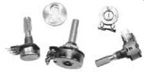
Fig. 2 Common potentiometer types.
Capacitors
Next to resistors, capacitors are probably the most common component in electronics. Capacitors are manufactured in a variety of shapes and sizes. In most cases, they are either flat, disk-shaped components; or they are tubular in shape. They vary in size from almost microscopic to about the same diameter, and twice the height, of a large coffee cup.
Capacitors are two-lead devices, sometimes resembling fixed resistors without the color bands.
Virtually all tube-shaped capacitors will have a capacitance value and a voltage rating marked on the body. Identification of this type is easy.
The small disk- or rectangle-shaped capacitors will usually be marked with the following code (where uF=microfarad):
Capacitor Markings
01-99 _ Actual Value in picofarads 101-0.0001 _F 331-0.00033 _F 102-0.001 _F 332-0.0033 _F 103-0.01 _F 333-0.033 _F 104-0.1 _F 334-0.33 _F 221-0.00022 _F 471-0.00047 _F
222-0.0022 _F 472-0.0047 _F 223-0.022 _F 473-0.047 _F 224-0.22 _F 474-0.47 _F With the previous coding system, a letter will usually follow the numeric code to define the tolerance rating. Tolerance, in the case of capacitors, is the allowable variance in the capacitance value. For example, a 10-_F capacitor with a 10% tolerance can vary by plus or minus (±) 1 _F. The tolerance coding is as follows:
Capacitor Tolerance-Markings
B _ ±0.1 pF J _ ± 5% C _ ±0.25 pF K _ ±10% D _ ±0.5 pF M _ ±20% F _ ±1% Z __80%, _20% G _ ±2%
Variable capacitors are, as the name implies, adjustable within a narrow range of capacitance value. The most common type is called the air dielectric type and is typically found on the tuning control of an AM (amplitude modulation) radio. Another type of variable capacitor is called a trimmer capacitor. These are usually in the range of 5 to 30 pF and are used for high-frequency applications.
Capacitor characteristics, functions, and additional parameter information will be discussed in Section 5. Some common shapes and sizes of capacitors are illustrated in Fig. 3.
Inductors
Inductors are broken down into two main classifications: transformers and chokes (or coils). Transformers designed for power conversion applications, called power transformers or filament transformers, are usually heavy, block shaped components consisting of two or more coils of wire wound around rectangular wafers of iron. Most of these types of transformers are intended to be mounted on a sturdy chassis because of their weight, but some newer types of split-bobbin power transformers are designed for printed circuit board mounting. Transformers designed for signal handling applications are smaller, and are usually mounted on printed circuit boards. Fig. 4 illustrates several common variations of transformers. Chokes are coils of wire either wound on a metallic core or a nonferrous form (to hold the shape of the coil).
Some types of small transformers and chokes are manufactured with an adjustable slug in the center. The slug is made of a ferrite material, and has threads on the outside of it like a screw. Turning the slug will cause it to move further into (or out of) the coil, causing a change in the inductance value of the coil or transformer. (Inductance is discussed in Section 3.) Depending on their application, these small adjustable inductors are called chokes, traps, IF transformers, and variable core transformers.
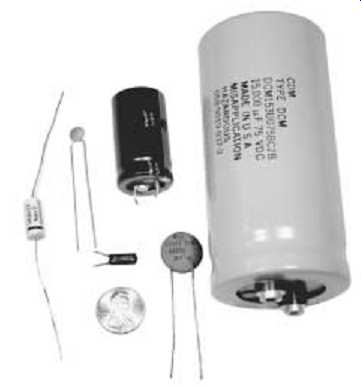
Fig. 3 Some examples of capacitors. The two larger capacitors are electrolytics.
Diodes
Diodes are two-lead semiconductor devices with tubular bodies similar to fixed resistors. Their bodies are usually either black or clear, with a single-colored band close to one end.
Diode bridges are actually four diodes encased in square or round housings. They have four leads, or connection terminals, two of which will be marked with a horizontal S symbol (sine-wave symbol), one will be marked "_" and the other "_." Several types of diodes and a diode bridge are illustrated in Fig. 5a.
Stud-mount diodes are intended for high-power rectification applications. They have one connection terminal at the top, a body shaped in the form of a hex-head (hexagonal-, i.e., six-sided-head) bolt (for tightening purposes), and a base with a threaded shank for mounting into a heatsink. (Heatsinks are devices intended to conduct heat away from semiconductor power devices. Most are made from aluminum and are covered with extensions, called fins, to improve their thermal convection properties.) Special types of diodes, called LEDs (the abbreviation for light-emit ting diodes), are designed to produce light, and are used for indicators and displays. They are manufactured in a variety of shapes, sizes, and colors, making them attractive in appearance. Fig. 5b illustrates a sampling of common LEDs. A specific type of LED configuration, called "seven-segment" LEDs, are used for displaying numbers and alphanumeric symbols. The front of their display surface is arranged in a block "8" pattern.
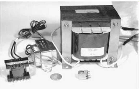
Fig. 4 A few examples of transformers. The small transformer in front
is an adjustable IF transformer.
Transistors
Transistors are three-lead semiconductor devices manufactured in a variety of shapes and sizes to accommodate such design parameters as power dissipation, breakdown voltages, and cost. A good sampling of transistor shapes and styles is illustrated in Fig. 6.
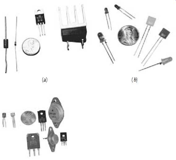
Fig. 5 (a) Two common diode types, a dual diode (three-lead device) and
a diode bridge (with the heatsink); (b) Common styles of light emitting diodes
(LEDs).
Fig. 6 Common transistor types.
Some power transistors have an oval-shaped body with two mounting holes on either side (this is called a TO-3 or TO-5 case style). At first glance, it appears to only have two leads, but the body itself is the third (collector) lead.
Integrated Circuits
Integrated circuits, or ICs, are multi-component semiconductor devices. A single IC might contain thousands of individual components manufactured through a series of special processes. They have multiple leads, called pins, which can vary in number from 8 to 40. ICs can be soldered directly into printed circuit boards, or plugged into specially designed IC sockets. Fig. 7 illustrates several varieties of integrated circuits.
Although the vast majority of integrated circuits have flat, rectangular bodies, a few types of ICs have round "can type" bodies similar to a common transistor case style. The difference is readily detectable by simply counting the number of lead wires coming from the can; a transistor will have three, but an IC of this style will have eight or more.
A Final Note on Parts Identification
If you think this is all rather complicated, you're right! This section covers only the most common types of components, and the easiest ways of identifying them and ascertaining their values. There are many more styles, types, and configurations than we have time or space to cover. A good way to build on this information is to open up some electronics supply catalogs and skim through them, paying special attention to the pictorial diagrams and dimensions relating to the various components. It will also be a great help to visit your local electronics supply store, and spend some time browsing through the component sales section. And, if it's any consolation, we still get stuck on a "what the heck is it" from time to time!
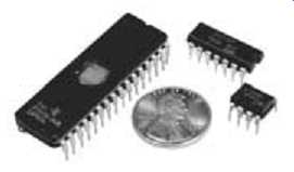
Fig. 7 Examples of integrated circuits. These are "dual in-line" (DIP)
styles.
Characteristics of Electricity
At some point in your life, you have probably felt electricity. If this experience involved a mishap with 120 volts AC (common household power from an outlet), you already know that a physical force is associated with electricity. You constantly see the effects of electricity when you use electrical devices such as electric heaters, television sets, electric fans, and other household appliances. You also see the effects of it when you pay the electric bill! But even with the almost constant usage of electricity, it often possesses an aura of mystery because it cannot be seen. In many ways, electricity is similar to other things that you do understand, and to which you can relate. Electricity follows the basic laws of physics, as do all things in our physical universe.
The electrical and electronics fields depend on the manipulation of subatomic particles called electrons . Electrons are negatively charged particles that move in orbital patterns, called shells, around the nucleus of an atom. Magnetic fields, certain chemical reactions, electrostatic fields, and the conductive properties of various materials affect the movement and behavior of electrons. As you progress through this guide, you will learn how to use electron movement and its associated effects to perform a myriad of useful functions in our lives.
As a beginning exercise in understanding electricity, you are going to compare it to something you can easily visualize and understand. Examine the simple water-flow system shown in Fig. 8. This hypothetical system consists of a water pump, a valve to adjust the water flow, and a water pipe to connect the whole system together. Assuming that the pump runs continuously and at a constant speed, it will produce a continuous and constant pressure to try to force water through the pipe.
If the valve is closed, no water will flow through the pipe, but water pressure from the running pump will still be present. The valve is totally "resisting" the flow of water.
If the valve is opened approximately half way, a "current" of water will begin to flow in the pipe. This will not be the maximum water current possible because the valve is "resisting" about half of the water flow.
If the valve is opened all the way, it will pose no resistance to the flow of water. The maximum water flow for this system will occur, limited by the capacity of the pump and the size (diameter) of the pipe.
The electrical circuit shown in Fig. 9 is very much like the water system shown in Fig. 8. Note the symbols used to represent a battery, resistor, switch, and wire. The battery is analogous to the pump. It provides an electrical pressure that produces an electrical flow through the wire. The electrical pressure is called voltage. The electrical flow is called current.
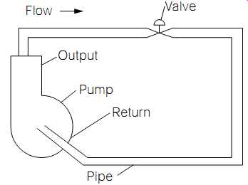
Fig. 8 Fluid analogy of an electric circuit.
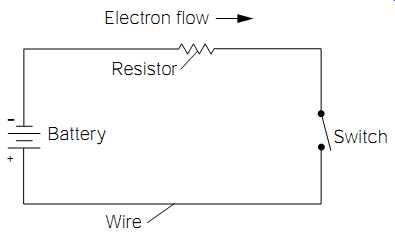
Fig. 9 Basic electrical circuit.
If the switch in Fig. 9 is open (in the "off" position), it will not allow current to flow because a continuous electrical path will not exist. This condition is analogous to the water valve (Fig. 8) being completely closed. Because a continuous electrical path from one side of the battery to the other does not exist with the switch open, this circuit is without continuity.
If the switch is closed (in the "on" position), an electrical current will begin to flow through the circuit. This current will start at the negative (- side of the battery, flow through the resistor (R1), through the closed switch (S1), and return to the positive (+ side of the battery. The wire used to connect the components together is analogous to the pipe (Fig. 8). The resistor poses some opposition to current flow, and is analogous to the water valve (Fig. 8) being partially closed. The actual amount of current flow that will exist in this circuit cannot be determined because we have not assigned absolute values to the components.
If the resistor was removed, and replaced with a piece of wire (assuming that the switch is left in the closed, or "on" position), there would be nothing remaining in the circuit to limit (or resist) the maximum possible current flow. This condition would be analogous to the water valve (Fig. 8) being fully opened. A maximum current would flow limited only by the capacity of the battery, and the size (diameter) of the wire.
Notice that in these two comparative illustrations, there is a device producing "pressure" (water pump or battery), a pathway through which a medium could flow (water pipe or wire), a device or devices offering "resistance" to this flow (water valve or resistor/switch combination), and a resultant flow, or "current," limited by certain variables (water pipe or wire diameter, water valve or resistor opposition, and water pump or battery capacity).
Simply stated, in any operational electrical circuit, there will always be three variables to consider: voltage (electrical pressure), current (electrical flow), and resistance (the opposition to current flow). These variables can now be examined in greater detail.
Voltage
Voltage does not move; it is applied. Going back to the illustration in Fig. 8, even with the water valve completely closed blocking all water flow, the water pressure still remained. If the water valve were suddenly opened, a water flow would begin and the water pressure produced by the pump would still exist. In other words, the water valve does not control the water pressure; only the water flow. The water pressure is an applied force promoting movement of the water. The water pressure does not move, only the water moves. The basic concept is the same for the electrical circuit of Fig. 9. The voltage (electrical pressure) produced by the battery is essentially independent of the current flow.
To help clarify the previous statements, consider the following comparison. Imagine a one-mile-long plastic tube with an inside diameter just large enough to insert a ping-pong ball. If this tube were to be completely filled from end to end with ping-pong balls and you inserted one additional ping-pong ball into one end, a ping-pong ball would immediately fall out of the other end. The force, or pressure, used to insert the one additional ping-pong ball was applied to every ping pong ball within the tube at the same time. The movement of the ping-pong balls is analogous to electrical current flow. The pressure causing them to move is analogous to voltage. The pressure did not move; it was applied. Only the ping-pong balls moved.
Voltage is often referred to as electrical potential, and its proper name is electromotive force. It is measured in units called volts. Its electrical symbol, as used in formulas and expressions, is E.
The level, or amplitude, of voltage is usually defined in respect to some common point. For example, the battery in most automobiles provides approximately 12 volts of electrical potential. The negative side of the battery is normally connected to the main body of the automobile, causing all of the metal parts connected to the body and frame to become the common point of reference. When measuring the positive terminal of the battery with respect to the body, a positive 12-volt potential will be seen.
The terms positive and negative are used to define the polarity of the voltage. voltage polarity determines the direction in which electrical current will flow. Referring to Fig. 8, note how the direction of the water flow is dependent on the direction, or orientation, of the water pump. If the pump had been turned around, so that the output and return were reversed, the direction of water flow would also have been reversed.
Another way of looking at this condition is to consider the output side of the pump as having a positive pressure associated with it; and the return, a negative pressure (suction) associated with it. The water will be pushed out of the output and be sucked toward the vacuum.
A similar condition exists with the electrical circuit of Fig. 9. The negative terminal of the battery "pushes out" an excess of electrons into an electrical conductor, and the positive terminal "attracts," or sucks in, the same number of electrons as the negative terminal has pushed out.
Thus, if the battery terminals are reversed, the direction of current flow will also reverse. (Note the symbol for a battery in Fig. 9. A battery symbol will always be drawn with a short line on one end and a longer line on the other. The short line represents the negative terminal; the long line represents the positive terminal.)
Current
Electrical current is the movement, or flow, of electrons through a conductive material. The fluid analogy of Fig. 8 showed some common principles of water flow. In the United States, the flow of water (and most other fluids) is measured in units as gallons per hour (gph). In the electrical and electronics fields, you need a similar standard to measure the flow of electrons. The gallon of electrons is called a coulomb. A coulomb is equal to 6,280,000,000,000,000,000 electrons, give or take a few! In scientific notation, that number is written 6.28 x 10^18 (6.28 with the decimal point moved 18 places to the right). Whenever one coulomb of electrons flows past a given point in one second of time, the current flow is equal to one ampere.
While on the topic of standards, let me provide you with the standard relationship between voltage, current, and resistance. One volt is the electrical pressure required to push one coulomb of electrons through one ohm of resistance in one second of time. In other words, 1 volt will cause a 1 ampere current flow in a closed circuit with 1 ohm of resistance. You will understand this relationship more clearly as you begin to work with Ohm's law.
The direction of current flow will always be from negative to positive. This is referred to as the electron flow. As stated previously, electron flow rate is measured in units called amperes, or simply amps. Its electrical symbol, as used in formulas and expressions is I.
As illustrated in Fig. 10, current can flow only in a closed circuit; that is, a circuit that provides a continuous conductive path from the negative potential to the positive potential. If there is a break in this continuous path, such as the open switch (S1) in Fig. 11, current cannot flow, and the circuit is said to be open. Another way of stating the same principle is to say the circuit of Fig. 10 has continuity (a continuous path through which current can flow). The circuit in Fig. 11 is without continuity.
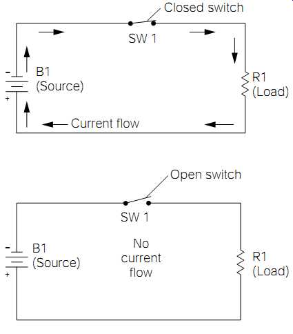
Fig. 10 Example of a closed circuit.
Fig. 11 Example of an open circuit.
Resistance
Resistance is the opposition to current flow. The open switch in Fig. 11 actually presents an infinite resistance. In other words, its resistance is so high, it doesn't allow any current flow at all. The closed switch shown in Fig. 10 is an example of the opposite extreme. For all practical purposes, it doesn't present any resistance to current flow and, therefore, has no effect on the circuit, as long as it remains closed.
The circuit illustrated in Fig. 10 shows the symbol for a resistor (R1) and the current flow (I) through the circuit. A resistor will present some resistance to current flow that falls somewhere between the two extremes presented by an open or closed switch. This resistance will normally be much higher than the resistance of the wire used to connect the circuit together. Therefore, under most circumstances, this wire resistance is considered to be negligible. Resistance is measured in units called ohms.
Its electrical symbol, as used in formulas and expressions, is R.
Alternating Current (AC) and Direct Current (DC)
The periodic reversal of current flow is called alternating current (AC).
In AC-powered circuits, the polarity of the voltage changes perpetually at a specified rate, or frequency. Because the polarity of the voltage is what determines the direction of the current flow, the current flow changes directions at the same rate. The symbol for an AC voltage is shown in Fig. 12.
The frequency of current alternations is measured in units called hertz (Hz). A synonym for hertz is cycles per second (cps). Both of these terms define how many times the current reverses direction in a one second time period. Common power of the average home in the United States has been standardized at 60 Hz. This means the voltage polarity and current flow reverse direction 60 times every second. (See Fig. 12.) In contrast to ac power sources (Fig. 12), a direct-current (DC) power source never changes its voltage polarity. Consequently, the current in a DC powered circuit will never change direction of flow. The battery power sources shown in Figs. 9 through 11 are examples of DC power sources, as are all batteries.
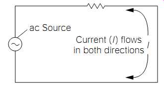
Fig. 12 Basic AC circuit illustrating current flow.
Conductance
Sometimes it is more convenient to consider the amount of current allowed to flow, rather than the amount of current opposed. In these cases, the term conductance is used. Conductance is simply the reciprocal of resistance. The unit of conductance is the mho (ohm spelled backward), and its electrical symbol is G. The following equations show the relationship between resistance and conductance (for example, 2 ohms of resistance would equal 0.5 mho of conductance, and vice versa):
1/G = R
The reciprocal of conductance is resistance
1/R=G
The reciprocal of resistance is conductance.
In the 1990s, the accepted term of conductance, mho, and its associated symbol G were replaced with the term siemen and its associated symbol S. These two terms, with their associated symbols, mean exactly the same thing. However, throughout the remainder of this guide, you will continue to use the older term mho, which is still the most commonly used method of expressing conductance.
Power
The amount of energy dissipated (used) in a circuit is called power.
Power is measured in units called watts. Its electrical symbol is P.
In circuits such as the one shown in Fig. 10, the resistance is often referred to as the load. The battery is called the source. This is simply a means of explaining the origin and destination of the electrical power used up, or dissipated, by the circuit. For example, in Fig. 10, the electrical power comes from the battery. Therefore, the battery is the source of the power. All of this power is being dissipated by the resistor (R1), which is appropriately called the load.
Laws of Electricity
As with all other physical forces, physical laws govern electrical energy.
Highly complex electrical engineering projects might require the use of several types of high-level mathematics. The electrical design engineer must be well acquainted with physics, geometry, calculus, and algebra.
However, if you do not possess a high degree of proficiency with high-level mathematics, this does not mean that you must abandon your goal of becoming proficient in the electrical or electronics fields. Many books are available on specific subjects of interest that simplify the complexities of design into rule-of-thumb calculations. Also, if you own a computer system, you can purchase computer programs (software) to perform virtually any kind of design calculations that you will probably ever need. Unfortunately, this doesn't mean that you can ignore electronics math altogether. The electronics math covered in this section is necessary for establishing and understanding the definite physical relationships between voltage, current, resistance, and power.
Ohm's Law
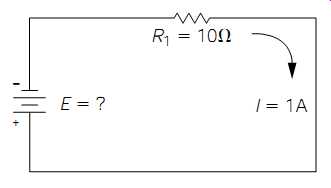
Fig. 13 Basic DC circuit illustrating Ohm' s law.
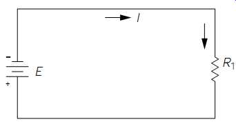
Fig. 14 Basic DC circuit.
The most basic mathematical form for defining electrical relationships is called Ohm's law. In the electrical and electronics fields, Ohm's law is a basic tool for comprehending electrical circuits and analyzing problems.
Therefore, it is important to memorize, and become familiar with, the proper use of Ohm's law, just as a carpenter must learn how to properly use a saw or hammer. Ohm's law is expressed as follows:
E =IR (eq. 1)
This equation tells us that voltage (E) is equal to current (I) multiplied by resistance (R). The simple circuit of Fig. 13 illustrates how this equation might be used. The value of R1 is given as 10 ohms (note the capital Greek omega symbol is used to abbreviate the word ohm), and the current flow is given as 1 amp, but the battery voltage (E) is unknown. By substituting the electrical symbols in Eq. (eq. 1) with the actual values, E can easily be calculated.
E =IR
E =(1 amp)10 ohms)
E =10 volts
Now you can go through a few more examples of using Ohm's law to really get the hang of it. Note the circuit illustrated in Fig. 14. We have not assigned any values to this circuit, so you can use the same basic circuit format to go through several exercises. If R is 6.8 ohms, and I is 0.5 amp, what is the source voltage?
E = IR
E = (0.5)(6.8)
E = 3.4 volts
If R is 22 ohms, and I is 2 amps, what would E be?
E = IR
E = (2)(22)
E = 44 volts
If R is 10,000 ohms, and I is 0.001 amp, what would E be?
E = IR
E = (0.001)(10,000)
E = 10 volts
Now consider some different ways you can use this same equation.
An important rule in algebra is that you might do whatever you want to one side of an equation, as long as you do the same to the other side of the equation. The principle is the same as with a balanced set of scales.
As long as you add or subtract equal amounts of weight on both sides of the scales, the scales will remain balanced. Likewise, you can add, sub tract, multiply, or divide by equal amounts to both sides of Eq. (1) with out destroying the validity of the equation. For example, divide both sides of Eq. (1) by R:
_ IR _ R E _ R
The two Rs on the right side of the equation cancel each other out.
Therefore:
_ I or I _ (eq. 2)
Equation ( 2) shows that if you know the voltage (E) and resistance (R) values in a circuit, you can calculate the current flow (I). Referring back to Fig. 13, you were given the resistance value of 10 ohms and the current flow of 1 amp. From these values you calculated the source voltage to be 10 volts. Assume, for the moment, that you don't know the current flow in this circuit. Equation ( 2) will allow you to calculate it:
I __ _ 1 amp
Now go back to the previous three exercises where you calculated voltage using Fig. 14 as the basic circuit. Assume the current flow value to be unknown, and using the known voltage and resistance, solve for current. In each exercise, the calculated current flow value should be the same as the given value.
Similarly, you could rearrange Eq. (1) to solve for resistance, if you knew the values for current flow and voltage. Note that each side of the equation must be divided by I:
_ The two Is on the right side of the equation cancel out each other, leaving
_ R or R _ (3)
Referring back to Fig. 13, assume that the resistance value of R1 is not given. Using Eq. (3), you can solve for R:
R __ _ 10 ohms
10 volts
_ 1 amp E _ I E _ I E _ I IR _ I E _ I 10 volts
__ 10 ohms E _ R E _ R E _ R
Once again, refer back to the exercises associated with Fig. 14, and assume that the value of resistance is not given in each case. Using Eq. (3) and the known values for current flow and voltage, solve for R. In each exercise, the calculated value of R should equal the previously given value.
At this point, you should be starting to understand what is meant by a proportional relationship between voltage, current, and resistance. If one of the values is changed, one of the other values must also change. For example, if the source voltage is increased, the current flow must also increase (assuming that the resistance remains constant). If the resistance is increased, the current flow must decrease (assuming that the source voltage remains constant), and so forth. For practice, you might try substituting other values for current, voltage, and resistance, using Fig. 14 as the basic circuit. It is vitally important to become very familiar with how this relationship works.
Parallel-Circuit Analysis
If Fig. 14 was an example of the most complex circuit you would ever have to analyze, you wouldn't need to go any further in circuit analysis.
Unfortunately, electrical circuits become much more complicated in real-world applications. But don't become discouraged; even extremely complicated circuits can usually be broken down into simpler equivalent circuits for analysis purposes.
Fig. 15 is an example of a simple parallel circuit. A parallel circuit is one in which two or more electrical components are electrically connected across each other. Note that resistors R1 and R2 are wired across each other, or in parallel. In a parallel circuit, the total current supplied by the source will divide between the parallel components. Note that there are two parallel paths through which the current might flow.
Before covering the calculations for determining current flow in parallel circuits, consider these functional aspects of Fig. 15.
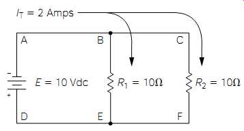
Fig. 15 Simple parallel DC circuit.
Electrically speaking, points A, B, and C are all the same point. Like wise, points D, E, and F are also at the same electrical point in the circuit.
Although this might seem confusing at first, remember that the wire shown in an electrical circuit diagram (electrical circuit diagrams are called schematics) is considered to have negligible resistance as compared to the rest of the components in the circuit. In other words, for convenience sake, consider the wire to be a perfect conductor. This means that point A is the exact same electrical point as point B because there is only wire between them. Point B is also the same electrical point as point C. From a circuit analysis perspective, the top of R1 is connected directly to the negative terminal of the battery. Likewise, the top of R2 is also connected directly to the negative terminal of the battery. This means that Fig. 15 can be redrawn into the form shown in Fig. 16. It is important to recognize that Fig. 15 and Fig. 16 are exactly the same circuit. (Because this concept is a little abstract, you might need to reread this paragraph and study Figs. 15 and 16 several times.)
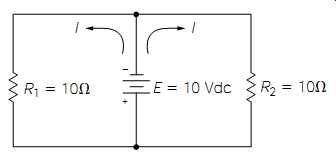
Fig. 16 The equivalent circuit of Fig. 15.
Fig. 16 makes it easy to see that both resistors are actually connected directly across the battery. Because the battery voltage is 10 volts DC, the voltage across both resistors will also be 10 volts DC. Now that two circuit variables relating to each resistor are known (the voltage across each resistor and its resistance value); Ohm's law can be used to calculate the current flow through R1:
I __ _ 1 amp
10 volts
__ 10 ohms E _ R
The previous calculation was for determining the current flow through R1 only. R2 is also drawing a current flow from the battery. It should be obvious that, because R2's resistance is the same as R1, and they both have 10 volts DC across them, the calculation for determining R2's current flow would be the same as R1. Therefore, you can conclude that 1 amp of current is flowing through R1, and 1 amp of current is flowing through R2. The battery in this circuit is a single source that must pro-vide the electrical pressure to promote the total electron flow for both resistors. Therefore, 2 amps of total current must leave the negative terminal of the battery, divide into two separate flows of 1 amp through each resistor, and finally recombine into the 2-amp total current flow before entering the positive terminal of the battery. This 2-amp total current flow is illustrated in Fig. 15.
Try another example. Referring back to Fig. 16, assume R1 is 5 ohms instead of 10 ohms. Note that the voltage across R1 will not change (regardless of what value R1 happens to be), because it is still connected directly across the battery. The current flow through R1 would be
I __ _ 2 amps
(R1 )(R2 )
__ (R1 ) _ (R2 ) 10 volts
_ 5 ohms E _ R
Now you have 2 amps flowing through R1, plus the 1 amp flowing through R2 (assuming the value of R2 remained at 10 ohms). The total circuit current being drawn from the source must now be 3 amps, because 2 amps are flowing through R1, and 1 amp is still flowing through R2.
As the previous examples illustrate, a few general rules apply to parallel circuits:
In a closed parallel circuit, the applied voltage will be equal across all parallel legs (or loops, as you think of them) In a closed parallel circuit, the current will divide inversely proportionally to the resistance of the individual loops (the term inversely proportional simply means that the current will increase as the resistance decreases, and vice versa) In a closed parallel circuit, the total current flow will equal the sum of the individual loop currents When analyzing parallel circuits, it is often necessary to know the combined, or equivalent, effect of the circuit instead of the individual variables in each loop. Referring back to Fig. 15, it is possible to consider the combined resistance of R1 and R2 by calculating the value of an imaginary resistor, Requiv. The following equation can be used to calculate the equivalent resistance of any two parallel resistances:
Requiv
_ (2-4)
By inserting the values given in Fig. 15, we obtain
Requiv
____ 5 ohms 100
_ 20 (10)(10)
__ (10) _ (10) (R1 )(R2 )
__ (R1 ) _ (R2 )
The 5 ohm (Requiv ) represents the total combined resistive effect of both R1 and R2. Because you already know the total circuit current is 2 amps, you can use Ohm's law to prove the calculation for Requiv is correct. Using Eq. (1), we have
E =IR =(2 amps)(5 ohms) =10 volts
Because it is true that the source voltage is 10 volts DC, you know that the calculation for Requiv is correct.
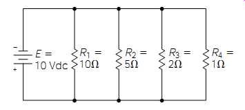
Fig. 17 Complex parallel circuit.
In circuits where there are three or more parallel resistances to consider, the calculation for Requiv becomes a little more involved. In these circumstances, a calculator is a handy little tool to have! You must calculate the individual conductance values of each resistor in the parallel net work, add the conductance values together, and then calculate the reciprocal of the total conductance. This sounds more complicated than it really is. Referring to the complex parallel circuit illustrated in Fig. 17, note that there are four resistors in parallel. To calculate Requiv , the first step is to find the individual conductance values for each resistor. For example, to find the conductance of R1:
G ___ 0.1 mho 1
_ 10 1
_ R
The conductance of the remaining resistors should be calculated in the same way. If you perform these calculations correctly, your conductance values should be:
G(R1) _ 0.1 (previous calculation) G(R2) _ 0.2
G(R3) _ 0.5 G(R4) _ 1
By adding all of the conductance values together, the total conductance value comes out to 1.8 mhos. The final step is to calculate the reciprocal of the total conductance, which is
[...]
for Fig. 17 is approximately 0.5555 ohms. Note that in the previous examples, Requiv is less than the lowest value of any single resistance loop in the parallel network. This will always be true for any parallel network.
The procedure for calculating Requiv in parallel circuits having three or more resistances can be put in an equation form:
(5)
When using Eq. (5), remember to perform the steps in the proper order as previously shown in the example with Fig. 17.
Series-Circuit Analysis
Fig. 18 Simple series DC circuit.
The circuit in Fig. 18 is an example of a simple series circuit. Notice the difference between this circuit and the circuit shown in Fig. 15. In Fig. 18, the current must first flow through R1, and then through R2, in order to return to the positive side of the battery. There can only be one current flow, and this flow must pass through both resistors.
In a series circuit, the combined effect of the components in series is simply the sum of the components. For example, in Fig. 18, the combined resistive effect of R1 and R2 is the sum of their individual resistive values: 10 ohms + 10 ohms = 20 ohms. In series circuits, this combined resistive effect is usually called Rtotal , although it might be correctly referred to as Requiv.
Knowing the total circuit resistance to be 20 ohms, and the source voltage to be 10 volts DC, Ohm's law can be used to calculate the circuit current (I total ):
I __ _ 0.5 amp 10 volts __ 20 ohms E _ R
In a series circuit, the current is the same through all components, but the division of the voltage is proportional to the resistance. This rule can be proved through the application of Ohm's law. The resistance of R1 (10 ohms) and the current flowing through it (I total = 0.5 amp) give us two known variables relating to R1. Therefore, R1's voltage would be
E =IR =(0.5 amp)(10 ohms) =5 volts
The 5 volts that appear across R1 in this circuit is commonly called its voltage drop. R2's voltage drop can be calculated in the same manner as R1's:
E =IR =(0.5 amp)(10 ohms) =5 volts
The fact that the two voltage drops are equal should come as no surprise, considering that the same current must flow through both resistors, and they both have the same resistive value.
If the voltage dropped across R1 is added to the voltage dropped across R2, the sum is equal to the source voltage. This condition is applicable to all series circuits.
A few general rules can now be stated regarding series circuits:
In a closed series circuit, the sum of the individual voltage drops must equal the source voltage.
In a closed series circuit, the current will be the same through all of the series components, but the voltage will divide proportionally to the resistance.
As has been noted previously, the resistors in Fig. 18 are of equal resistive value. However, in most cases, components in a series circuit will not present equal resistances. To calculate the voltage drops across the individual resistors, you might use Ohm's law as in the previous example. Another way of calculating the same drops is by using the ratio method. To us e the ratio method, calculate Rtotal by adding all of the individual resistive values.
Make a division problem with Rtotal the divisor, and the dividend the resistive value of the resistor for which the voltage drop is being calculated. perform this division, and then multiply the quotient by the value of the source voltage. The answer is the value of the unknown voltage drop.
Referring to Fig. 19, assume you desire to calculate the voltage drop across R1 using the ratio method. Start by finding Rtotal:
Rtotal
_ R1
_ R2
_ R3
_ 2 ohms _ 3 ohms _ 5 ohms _ 10 ohms
Next, make a division problem with Rtotal as the divisor and R1 as the dividend and perform the division:
_ 0.2 2 ohms
__ 10 ohms
Finally, multiply this quotient by the value of the source voltage:
(10 volts)(0.2) _ 2 volts
The voltage dropped across R1 in Fig. 19 will be 2 volts. As an exercise, calculate the voltage drop across R1 using Ohm's law. You should come up with the same answer.
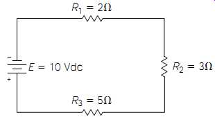
Fig. 19 Series circuit with unequal resistances.
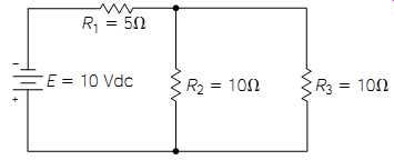
Fig. 20 Example of a series parallel circuit.
Series-Parallel Circuits
In many situations, series and parallel circuits are combined to form series-parallel circuits (Fig. 20). In this circuit, R2 and R3 are in parallel, but R1 is in series with the parallel network of R2 and R3. If this is con fusing, notice that the total circuit current must flow through R1, indicating that R1 is in series with the remaining circuit components.
However, in the case of R2 and R3, the total circuit current can branch; with part of it flowing through R2, and part of it flowing through R3.
This is the indication that these two components are in parallel.
To analyze the circuit of Fig. 20, you would start by simplifying the circuit into a form that's easier to work with. As previously explained regarding parallel circuits, resistors in parallel can be converted to an Requiv value. In this case, R2 and R3 are in parallel, so Eq. (4) might be used to calculate Requiv:
Requiv
____ 5 ohms 100
_ 20 (10)(10)
__ (10) _ (10) (R1 )(R2 )
__ (R1 ) _ (R2 )
Once the value of Requiv is known, the circuit of Fig. 20 can be redrawn into the form illustrated in Fig. 21. You should recognize this as a simple series circuit. Rtotal can be calculated by adding the values of R1 and Requiv:
Rtotal
_ R1
_ Requiv
_ 5 ohms _ 5 ohms _ 10 ohms
Using the values of Rtotal , and the source voltage, Ohm's law can be used to calculate the total circuit current (I total ):
I __ _ 1 amp 10 volts
__ 10 ohms E _ R
The voltage drop across R1 can be calculated using the variables associated with R1 (I total and R1):
E =IR =(1 amp)(5 ohms) =5 volts
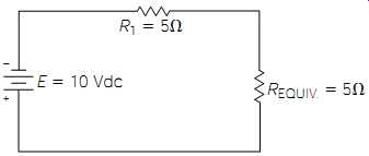
Fig. 21 Simplified equivalent circuit of Fig. 20.
In this particular circuit, you can take a shortcut in determining the voltage drop across Requiv. Because you know that the individual voltage drops must add up to equal the source voltage in a series circuit, you can simply subtract the voltage drop across R1 from the source voltage, and the remainder must be the voltage drop across Requiv:
10 volts (source) - 5 volts (R1) = 5 volts (Requiv )
As stated previously, the applied voltage (in a parallel circuit) is the same for each loop of the circuit. Because you know that 5 volts is being dropped across Requiv , this actually means that 5 volts is being applied to both R2 and R3 in Fig. 20. Now that two variables are known for R2 and R3 (the voltage across them, and their resistive value), the current flow through them can be calculated. Calculating the current flow through R2 first:
I __ _ 0.5 amp 5 volts __ 10 ohms E _ R
Obviously, with the same resistive value and the same applied voltage, the current flow through R3 would be the same as R2. Knowing that the individual current flows in a parallel circuit must add up to equal the total current flow, you can add the current flow through R2 and R3 to double check our previous calculation of I total:
0.5 amp (R2 ) _ 0.5 amp (R3 ) _ 1 amp
Power
An important variable to consider in most electrical and electronics circuits is power. Power is the variable which defines a circuit's ability to perform work. Electrical power is dissipated (used up) in the forms of heat and work. For example, the majority of electrical power used by a home stereo is dissipated as heat, but a good percentage is converted to acoustic energy (varying pressure waves in the air which is called sound).
It is often necessary to calculate the amount of power that must be dissipated in a circuit or component to keep from destroying something.
Also, if you are supplying the power to a circuit, you need to know the amount of power to supply. The following three equations are used for power calculations:
P _ IE ( 6)
Power is equal to the current multiplied by the voltage:
P _ I 2 R ( 7)
Power is equal to the current squared, multiplied by the resistance:
P _ ( 8)
E 2 _ R
Power is equal to the voltage squared, divided by the resistance.
Examine how these equations could be used to calculate the power dissipated by R1 in Fig. 18. (Remember, you calculated the voltage drop across R1 to be 5 volts in an earlier problem.) Using Eq. (6) and the known variables for R1:
P _ IE _ (0.5 amp)(5 volts) _ 2.5 watts
Using Eq. (7) and the known variables for R1:
P _ I 2 R _ (0.5 amp)(0.5 amp)(10 ohm) _ 2.5 watts
Using Eq. (8) and the known variables for R1:
P __ _ 2.5 watts (5 volts)(5 volts)
__ 10 ohms E 2
_ R
As you can see from the previous calculations, you need to know only two of three common circuit variables (voltage, current, and resistance) to solve for power.
There is a very important point to keep in mind when performing any electrical or electronic calculation; don't mix up circuit variables with component variables. For example, in the previous power calculations, the power dissipated by R1 was solved for. To do this, you used the voltage across R1, the current flowing through R1, and the resistance value of R1. In other words, every variable you used was "associated with R1." If you wanted to calculate the power dissipated by the entire circuit of Fig. 18, you would have to use the variables associated with the entire circuit. For example, using Eq. (8) and the known circuit variables:
P __ _ 100/20 _ 5 watts (10 volts)(10 volts)
__ 20 ohms E 2
_ R
Notice that the voltage used in the previous equation is the source voltage (the total voltage applied to the circuit), and the resistance value used is Rtotal (R1 + R2 ; the total circuit resistance).
Our answer, therefore, is the power dissipated by the total circuit.
Common Electronics Prefixes
Throughout this section, the example problems and illustrations have used low value, easy-to-calculate values for the circuit variables. In the real world, however, you will need to work with extremely large and extremely small quantities of these circuit variables. Because it is cumbersome, and both space- and time-consuming, to try to work with numbers that might have 12 or more zeros in them, a system of prefixes has been standardized. These prefixes, together with their associated symbols and values are:
Electronic Prefixes
pico (symbol "p") _ 1/1,000,000,000,000 nano (symbol "n") _ 1/1,000,000,000 micro (symbol "_") _ 1/1,000,000 milli (symbol "m") _ 1/1,000 kilo (symbol "K") _ 1,000 mega (symbol "M") _ 1,000,000
Notice that prefixes for numbers greater than one are symbolized by capital letters, but symbols for prefixes of less than one are lowercase letters. Also, note that the Greek symbol _ (pronounced "mu") is used as the symbol for micro, instead of "m," to avoid confusion with the symbol used for the prefix "milli."
The following list provides some examples of how prefixes would be used in conjunction with common circuit variables. The abbreviation provided with each example is the way that value would actually be written on schematics or other technical information.
EXAMPLES
1 picovolt _ 0.000000000001 volt (abbrev. 1 pV) 15 nanoamps _ 0.000000015 amp (abbrev. 15 nA) 200 microvolts _ 0.0002 volt (abbrev. 200 _V) 78 milliamps _ 0.078 amp (abbrev. 78 mA) 400 Kilowatts _ 400,000 watts (abbrev. 400 KW) 3 Megawatts _ 3,000,000 watts (abbrev. 3 MW)
Using Ohm's Law in Real-World
Circumstances
Thus far, you have been exposed to the basic concept of Ohm's law and how circuit variables have a definite and calculable relationship to each other. As you have seen, the mathematics involved with Ohm's law are not difficult, but it takes some practice to become proficient at applying Ohm's law correctly. For example, in the early stages of becoming accustomed to using Ohm's law, it is a common error to mistakenly mix up (or confuse) circuit variables with individual component variables. It is also easy to misplace a decimal point when working with the various standardized prefixes (milli, micro, Mega, etc.).
When electronics professionals draw a complete circuit diagram of a complex electronic system, usually referred to as a schematic, they often complicate the easy visualization of circuit subsections in the effort to make the complete schematic fit into a nice, neat, aesthetically pleasing square or rectangle. This means that the electronics enthusiast must become proficient at being able to visualize a parallel circuit, for example, drawn horizontally, vertically, or in any number of possible configurations. In other words, it is necessary to develop the ability to conceptualize a schematic, which means merely being capable of mentally simplifying it into familiar subsections that can be easily worked with.
This is a learned talent, and the more time you spend at conceptualizing schematics, the more skilled you will become.
The purpose of this section is to familiarize you with using Ohm's law in conjunction with more typical real-world circuits. The following exercises are designed to help you become acquainted with the following areas of difficulty:
1. Using Ohm's law correctly
2. Becoming familiar with commonly used prefixes
3. Simplifying more complex schematic diagrams
In addition, you will examine the following exercises in several ways.
First, you will go through each exercise, working out the electrical problems, and developing the aforementioned skills. Next, you will go through the exercises a second time, examining the real-world component values that could be inserted into these circuits to make them practical to construct and test. As a final, optional, exercise, you may want to purchase the materials at a local electronics store to literally construct and test these circuits. The only components required will be a handful of resistors, a 9-volt battery (the small, rectangular type), and a few general-purpose LEDs (i.e., light-emitting diodes). All these circuits can be easily constructed using clip leads. The total cost of the components should be less than $10.00 (it is assumed that you already have a good DVM and an adequate supply of clip leads-these are part of your basic lab supplies, and will be used over and over). If you have not yet purchased a DVM or the majority of your lab supplies, you can always come back to this section and acquire some hands-on experience with building these circuits at a later time.
Electrical Calculations (Ideal)
The most common method of analyzing electrical circuits is to consider all of the circuit components and circuit variables to be "ideal." In real life, various circuit variables, such as battery voltages, resistor values, and other component values, are not exact.
The simple fact that virtually all electronic components are specified as having a tolerance (i.e., an allowable variance from an exact specification) indicates that calculated circuit variables will always contain some error depending on how broad the accepted tolerance values are. In other words, a 10-ohm resistor dropping 10 volts would be expected to conduct 1 amp of current (10 volts divided by 10 ohms =1 amp). This is an ideal calculation. However, if the resistor were specified as being 10 ohms with a 10% tolerance, its actual value could range between 9 and 11 ohms, causing the actual, or real-life current flow to be between 1.11 and 0.909 amps. Unfortunately, there isn't any method of determining actual circuit variables without literally constructing the circuit and measuring the variables. Even in doing so, the actual circuit variables could be different in two identical circuits, as a result of the unpredictable effects of component tolerances. Consequently, the only practical method of analyzing circuits is to consider all of the circuit conditions to be "ideal." This simply means considering such things as component values and source voltages to be exactly as specified. You will also consider all inter connecting wiring and wiring connections to be ideal, or representing "zero" resistance. This is really no different from a carpenter drawing blueprints for a construction project, assuming the available lumber to be straight and dimensionally accurate.
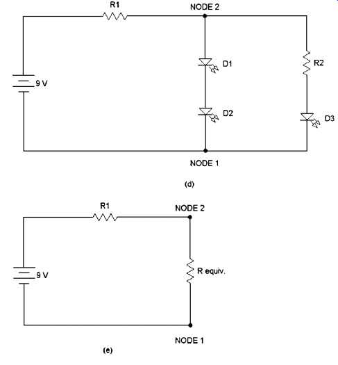
All of the circuit diagrams used for the following exercises contain one or more LEDs. Light-emitting diodes are most commonly used to provide a visual light for indication purposes. You will learn more about the theory and physics of LEDs in Section 7, but for now, you will only need to remember a few basic characteristics and approximations.
First, the current flow through an LED must be in the proper direction for it to produce visible light. In other words, if you build any of the following circuits and connect the LED backward in the circuit, it will not light. The low voltages used in these circuits will not harm the LED, so if it doesn't light, simply try reversing the leads. Second, it will be assumed that all of the LEDs in the following exercises will drop 2 volts, and they will require 10 milliamps (i.e., 0.01 amp) of current flow to light. These LED specifications are close enough to be applicable to the majority of general-purpose LEDs.
Fig. 22 Circuit diagram examples for practice problems using Ohm' s law.
NOTE: I chose this technique of using a few LEDs, resistors, and 9-volt battery for several reasons. First, we all like to occasionally take a break, get away from the books, and physically work with something related to what we have learned. Ohm's law can be learned academically, and it can be aptly demonstrated using only a power source and a few resistors; however, the circuit doesn't appear to "do" anything.
In our experience, it is more fun and memorable if an experimental circuit performs some practical function, even if that function is as simple as lighting an LED.
Exercise 1 Fig. 22a illustrates a 9-volt battery connected to a resistor (R1) and an LED (D1) (Note the two small arrows pointing away from D1. This is the typical method of drawing the schematic symbol for an LED-the two arrows symbolizing the light emitted by the LED.) You should recognize this circuit as a simple series circuit, since the same current flow must flow through all of the components (i.e., the current cannot "branch" into any other circuit legs).
Remembering the aforementioned approximations for all general-purpose LEDs, you know that you want 10 milliamps of current to flow through the LED, and you also know the LED will drop 2 volts. As a beginning exercise, use Ohm's law to calculate the value of R1. (Don't worry if you're a little confused at this point. You'll get the hang of it as you proceed through a few more of these exercises.) The same current must flow through all of the components in a series circuit. Therefore, if the current flow through the LED is 10 milliamps, the current flow through R1 must be 10 milliamps. All the voltage drops in a series circuit must add up to equal the source voltage. In this example, the source voltage is the 9-volt battery. If the LED is drop ping 2 volts, this means that R1 must be dropping 7 volts (i.e., 9 volts _ 2 volts _ 7 volts). Now you know two electrical variables that specifically relate to R1: the current flow through it (10 milliamps) and the voltage drop across it (7 volts). Ohm's law states that the resistance value of R1 will equal the voltage dropped across it divided by the current flow through it. Therefore:
R __ _ 700 ohms
7 _ 0.01 E _ I
Of what practical value is this exercise? Suppose you wanted to con struct an illuminated Christmas tree ornament using a single LED and a 9-volt battery (such ornaments are commonly sold at exorbitant prices).
You now know how to choose an appropriate "limiting" resistor so that the maximum current specifications of the LED are not exceeded.
If you physically construct this circuit for experimental purposes, you can also use it to test an unknown grab-bag assortment of LEDs. R1 can be a common 680-ohm resistor. If some LEDs won't light (assuming that you have already tried reversing the connections), it is possible that they are special-purpose LEDs with internal limiting resistors. Put these aside for future use and categorization after you read and understand more about LEDs in Section 7.
Fig. 23 Circuit diagram examples for practice problems using Ohm' s law.
Fig. 23 (Continued)