AMPLIFIER SPECIFICATIONS
THE SPECIFICATION of a hi-fi amplifier is composed of numerous parameters, which may go something like this:
Power Output 25+25W r.m.s. 1kHz
8 ohms; 35+35W r.m.s. 1kHz
4 ohms; 20+20W r.m.s.
40 Hz -20kHz; 75W music.
Harmonic Distortion 1% total at rated power; 0.1% at half (-3d B) rated power.
intermodulation Distortion
0.2% at half rated power (60Hz: 7kHz= 4: 1).
Power Bandwidth 20Hz -40kHz.
Frequency Response 20Hz -30kHz (± 1dB).
Damping Factor 30 ref. 8 ohms and 1kHz.
Hum and Noise (volume control zero)
1mV maximum.
Signal-to-noise (S/ N) Ratio
Phono 66dB. Auxiliary 70dB. Tape 75dB.
Input Sensitivity and Impedances
Phono 2 · 5mV (47k-ohml.
Auxiliary 200mV ( 100k-ohm). Tape 200mV (100k-ohml.
Phono Overload 100mV r.m.s. for 0.5% distortion.
Tape Recording Output 20mV pin (40mV DIN).
Tone Controls Bass± 10dB at 100Hz.
Treble±10dB at 10kHz.
Loudness
+B dB at 100Hz and+4<:!_!!at 10kHz with volume control. set to -30dB.
Filters Low 30Hz and 12dB/octave.
High 7kHz and 6dB/ octave.
Mains Input
240V50Hz.
The parameters may not be expressed exactly like this and there may be fewer or more of them, depending on the method of testing and on the quality and cost of the amplifier and on the facilities provided. The best way of getting to grips with these parameters is to run through them in turn to see how they can be interpreted. After this the plan will be to investigate the parameters in terms of home requirements.
Power Output
The first on the list, the power output, is a primary parameter of an amplifier.
It tells how much urge the amplifier can provide under certain conditions and is akin to the horsepower rating of a motor car.
When you buy an electric light bulb or electric fire the main parameter that you particularly look out for is the wattage rating. So it is with a hi-fi amplifier, but in this case it is the power supplied rather than the power dissipated; it is determined as per the simple illustration of power in Section 1.
The amplifier is loaded by a large resistor of a suitable power rating (this is· called the output load), a continuous (sinewave) signal of a specified frequency is coupled to an input of the amplifier and the voltage across the load is measured while it is simultaneously being monitored on an oscilloscope and (possibly) distortion factor meter.
With a stereo amplifier both of the channels are so loaded and driven (the four of a quadraphonic one). This is implied by the example parameter of 25 ±25W. In this case the loads are 8 ohms. The input drive signal is increased until either the peaks of the sinewave are just about to clip or the distortion on the output signal reaches a datum value (usually 0.5% or 1 %), which signifies that the full power of the amplifier has been reached at that particular frequency. Increasing the drive beyond this point merely increases the clipping and hence the distortion.
The example shows that each channel will yield 25W into an 8-ohm resistive load when the two channels are working together at 1kHz for a distortion of 1% (just at peak clipping). Note that the distortion is indicated by the second parameter quoted and that in this example 25+25W is referred to as the rated power; also that this power is available at 1kHz only.
RMS Voltage
Recalling the simple power calculations in Section 1, it will be understood that the voltage across 8-ohm for 25W power is equal to the square root of the product of the power and the load resistance (i.e., V= yWR), which works out to 14 ·14V. Thus at the peak clipping point this voltage will be measured across each 8-ohm load.
This is the root mean square (r.m.s.) voltage of a sinewave. The 240V of our mains supply is also the r.m.s. voltage. It is the voltage measured on a r.m.s. voltmeter and it is equivalent to the heating power of a d.c. voltage (i.e., from a large battery) of the same value. A sinewave, though, also has a peak value, which is y2 times the r.m.s. voltage. Thus the peak value of 240V mains is 339.41 V. From the positive to the negative peak the peak-to-peak value is
678.82V! Sine 45• = 0•707
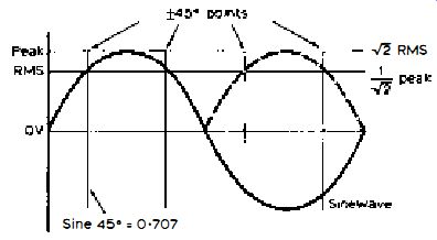
Fig. 2.1: Primary parameters of a sinewave (see text) . Some of the primary
parameters of a sinewave are shown in Fig. 2.1. Here we see that the r.m.s.
value occurs at four points only when the angles are ±4S degrees and the
sine value is 0.707 (i.e., 1/radical 2). At any point over a sinewave the
instantaneous voltage or the instantaneous current can range from zero
to the peak value of the waveform. Likewise the power. Into a resistive
load, therefore, the power is 0 W at the instant when both V and I are
zero and peak W at the instant when V and I are peak.
Average Power
Using the 14.14V across 8-ohm of the exampled 25+25 W amplifier, the peak of 14.14V r.m.s. is pretty well 20V. Using this peak voltage in the power calculation we get 50 W - not 25 W. Thus, the power ranges from zero to 50W peak, so the average power is 25W, so that when the r.m.s. voltage is used in the power calculation the result is the average power. This is sometimes erroneously given in the spec as the 'r.m.s. power'. Whenever you read 'r.m.s. power' in a spec. therefore, think average power! If you ever see a spec with a peak power parameter halve it to get to the real, average power. At one time dodges and artifices such as this were adopted by the ad people to give the false impression of the amplifier being more powerful than a competitor's of possibly lesser, real average power.
Happily, the Trade Descriptions Act of 1968 has put a penalty on such sharp practices! But still be on the lookout yourselves.
Load Values
Contemporary transistor amplifiers are constant voltage devices. This means that the voltage across the load holds fairly constant over a range of load values right down to the lowest value load that the amplifier is designed to accommodate. This results from the use of heavy negative feedback and the resulting low source resistance (see under 'Damping Factor'). The spec may well indicate a range of load values, corresponding to the impedances of latter-day loudspeakers (for the amplifier is designed ultimately to drive a loudspeaker - not to heat resistors or light electric light bulbs!). The example parameter indicates a maximum output of 14.14V r.m.s. across 8 ohm (giving 25W average power for each channel). If it is assumed that this voltage holds across 4 ohm, then, of course, the power is double or 50W. If the load is 16 ohm, then the power is halved (12.5W). Current Limiting In spite of the low source resistance of the amplifier, the voltage to peak clipping does tend to fall slightly as the load is reduced, which is why the example parameter shows 35+35W into 4-ohm loads, instead of the expected 50+50W. Nevertheless, the power into the load does rise as the load value is decreased.
The current through the load also rises, of course, as its value is reduced, and as excessive current can blow the output transistors, current limiting is often included in the design, which is another reason why the power does not always double when the load resistance is halved. If there was no such limiting (or fusing) the current would rise infinitely if a short circuit happened to occur across the loudspeaker or wiring under full drive.
Thus, when comparing amplifiers for power yield always make sure that you are comparing like with like. That is, that the comparison is made at a common load value -4 ohm or 8 ohm, whichever is the most convenient.
Frequency Range
So far we have investigated the power parameter at 1kHz only. These days amplifiers are expected to deliver their rated power over a frequency range from 20Hz -20kHz, or thereabouts. Not all amplifiers are capable of delivering the power available at 1kHz over the whole frequency range.
In the example parameter it will be seen that over 40Hz-20kHz the power is down to 20+20W. It would undoubtedly be even less than this at 20Hz. In this case the spec writer has deliberately restricted the low-frequency to avoid having to derate the power too much (i.e., over 20Hz-20kHz it may be 12+ 12W!). It will also be noticed that a load value is not given for this part of the parameter. Always regard with great suspicion any parameter which is incomplete.
Thus when comparing amplifier powers always make sure that you are comparing the powers at a common frequency or over a common frequency range. For example, a parameter going something like
25+25W 8 ohm
20Hz-20kHz is better than one going 25+25W 8 ohm
40Hz-20kHz and far better than one going 25+25W 4 ohm 40Hz-20kHz.
Music Power
The term 'music power' is sometimes included in the power parameter. It is not very meaningful and is less used nowadays . It shows how much relative power the amplifier can deliver on music type signal as distinct from continuous sinewave signal . The measurement is made using 'chopped' signal , and because the output is not then continuous (the amplifier having a little time- to recover between 'bursts') the effective power capability is often increased over the average power, but this depends on the design and adjustment of the power amplifier, including the size of heat sinks used for the output transistors, and on the nature of the power supply.
Moreover, the music rating is commonly expressed as that power of the two stereo or four quadraphonic channels added together . For example, if the average power of an amplifier is given as, say, 25+25W, then the music power would be 50W plus the extra which is available due to the use of a non-sinewave signal , which could add another 20% or more to the average power rating.
It should always be remembered that the average power of an amplifier is the same sort of power that lights our bulbs and runs our electric fires . It differs in frequency, of course; in the UK the mains frequency is 50Hz (60Hz in American countries) , which is at the low-frequency end of the audio spectrum - near 02 on the piano (the eleventh key up from the bass end) . Our amplifiers are expected to supply power from the low-frequency of 20Hz or so up to, at least , 20kHz; that is, a range of three decades or ten octaves, at least ! While mains power into a bulb or electric fire is continuous at the particular wattage rating, amplifier power fluctuates widely on music signal. By feeding an amplifier channel with continuous sinewave signal and connecting a bulb in place of the loudspeaker, the bulb would glow continuously and brightly when its voltage and wattage ratings correspond to those of the amplifier . Feeding the amplifier channel with music signal , from a gramophone pickup or radio tuner, for example, the bulb illumination would pulsate in sympathy with the music. Our amplifiers , of course, are not designed for this.
Their job is to supply current to the connected loudspeakers .
Amplifier /Loudspeaker Interface
While loudspeakers are current operated, their sensitivity in terms of sound pressure output at a given distance and under stipulated conditions is referred to an input voltage of shaped noise signal which has some of the features of music signal . The actual power abstracted by a loudspeaker partly depends on its modulus of impedance (Z). Section 6 gives information on this, but some aspects of the amplifier /loudspeaker interface will be best looked at now.
It has already been noted that a hi-fi , negative feedback amplifier represents a constant voltage source. Thus, at a given output voltage the current flowing through a connected loudspeaker depends on Z. Impedance Z means that the load includes reactive components (i .e. , capacitance and inductance) .
The value of Z is therefore not constant over the frequency range, as pure resistance (R) is. It is usually the value measured at 40Hz or 1kHz - called the nominal impedance. At the low-frequency resonance of the loudspeaker Z can rise a number of times above the nominal impedance - called the motional impedance. There may also be other, less dramatic peaks and troughs at higher frequencies, depending on the overall system design and the frequency-dividing networks used.
The current, and hence the power, thus falls when Z rises and rises when Z falls. For this reason alone it is virtually impossible to calculate the average power taken by the loudspeaker on wide-band signal.
Power Factor
Another reason why the power delivered to a loudspeaker is not as would be expected from the impedance is because owing to the reactive components of the load the current through it and the voltage across it do not rise and fall precisely in step at all frequencies. We have seen ( Section 1) that with a pure R load the power is W = VI. With a Z load the power is W = Vlcos0, where cos θ is the cosine of the angle of lead or Jag of the current with respect to the voltage, which is the power factor.
At some frequencies the 0 of certain loudspeakers can swing to 40-60 degrees. Assuming a swing of 60 degrees, the cosine of this is 0 · 5, which means that the power is half that which would be produced into a pure R load, when the Z and R values are the same! Moreover, if the 0 is large when the Z is low, some amplifiers are 'triggered' into current limiting before the maximum voltage that can be obtained across a pure R load is reached, which, of course, puts a limit on the maximum sound pressure output relative to a given level of distortion.
For these reasons, therefore, it would be far better to have our amplifiers rated in output voltage across specified loads rather than in output power, which merely signifies the potency of the amplifier in heating pure resistance!
Distortion
This parameter was introduced in the foregoing section. When the rated output of an amplifier is reached the distortion is round 0.5 to 1 % corresponding to the threshold of peak clipping. Any attempt to increase the output would result in a swift and considerable rise in distortion.
Fig. 2.2 oscillograms depict sinewave signal on one trace at a level causing severe clipping of one peak and music signal at three levels on the other trace.
Low level music well below clipping is shown at (a). Higher level music but still below clipping is shown at (b). Much higher level music this time taking the amplifier into peak clipping is shown at (c). While (a) and (b) would give a palatable sound, (d) would be very rough and disconcerting. Below the rated output (a) and (b) the distortion should be very small. The example spec shows a distortion of only 0 · I % at half (-3dB) the rated output.
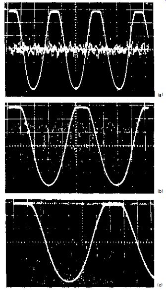
Fig. 2.2: Oscillograms showing peak-clipped sinewave on one trace and
music signal on the other trace. (al Low level music signal well below
clipping. (b) Higher level music signal but still below clipping. (c) Very
high level music signal running into peak clipping and hence severely distorted
.
Harmonic Distortion
This is harmonic distortion which is measured by applying a very pure ( distortion free) sinewave input at the required frequency and turning up the output for the required voltage across the load. A special instrument (distortion factor meter) is then used to delete the fundamental so that only the sum of all the harmonics and noise components remains. This is then compared in terms of a voltage ratio or percentage with the original output voltage.
For example 0.1 % means that the summed voltage of the harmonics and noise components is 1,000 times less than the voltage of the fundamental. If the fundamental corresponds to 20V, then the harmonics, etc. would correspond to a mere 20mV (i .e. , 0.02V) . There are other ways of measuring harmonic distortion with a wave or spectrum analyzer (see Audio Technician's Bench Manual). Some of the latest top-flight amplifiers boast an even lower distortion, but the percentage distortion is often related to frequency, usually being less at 1kHz than at low and high frequencies at the spectrum extremes.
A clipping amplifier produces a whole train of harmonics . Based on a 1kHz fundamental, we get the second at 2kHz, the third at 3kHz, the fourth at 4kHz, etc. Some of the higher order, odd harmonics are much more disconcerting than higher level low order, even harmonics. A fair measure of second and possibly third harmonic distortion can be tolerated, but dissonant harmonics referred to middle C and taken as 250Hz for convenience include the seventh at 1,750Hz, the ninth at 2,250Hz, the eleventh at 2,750Hz and other odd ones up to about the twenty-fifth at 6,250Hz. All these are less liked by the ear even when their amplitudes are less than those of lower order , even harmonics.
(a) (b)
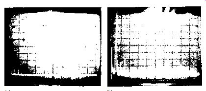
Fig. 2.3: Harmonic spectrograms ref. 1kHz 0-dB driving signal. (a) Very
good result showing second and third harmonics at -83dB (. (J07%J. (b)
Less dramatic though good result showing second harmonic at -75dB (0· 017%)
and third harmonic at -96dB (0·035%), with spurious signal of -80dB (0.01
%) at 16kHz. Scale 10dB/2kHz/ div.
(a) (b)
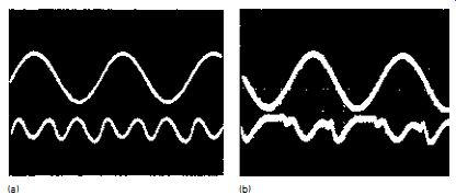
Fig. 2.4: Distortion factor oscillograms with the driving sinewave on
one trace and the residual on the other trace. (a) Mostly second and third
harmonic. (b) Showing crossover distortion and the resulting high order
harmonic (see text for evaluation) . Spectral Analysis A well designed
amplifier operating below clipping produces mostly second and third harmonics
, and a couple of examples are given in Fig. 2.3, (a) showing the remarkable
result from the Pioneer SA990 amplifier, where the second and third harmonics
are each at the astonishingly low level of -83dB (0.007%), and (b) a less
dramatic but nevertheless good result of -75dB (0.017%) second and -69dB
(0.035%) third, with a -80dB (0.01 %) spurious signal at 16kHz.
Only this sort of spectral analysis can identify the individual harmonics , spurious signals and their amplitudes with respect to the driving signal , which is 1kHz in the examples set to 0-dB datum.
The sum of the harmonics and noise from the output of a distortion factor meter is shown merely as a waveform on an oscilloscope, but the nature of the waveform sometimes gives a clue as to the order of the harmonics. Examples are given in Fig. 2.4, (a) where the harmonics are low order (mainly second and third) , and (b) where the 'peaky' parts of the distortion waveform indicate higher order components.
Display (b) , in fact, indicates the presence of so-called crossover distortion which occurs in some transistor amplifiers at low output owing to Incorrect biasing or poor design of the power amplifiers . This distortion, being of high order, is dissonant . At low volume, therefore, the amplifier responsible for (b) would possibly audition less favorably than the amplifier responsible for (a) , even though the distortion factor percentage might be far greater at (a) than at (b) . This kind of detailed distortion information is rarely given in manufacturers' specifications , but it can be found in the comprehensive reviews published by reputable hi-fi magazines.
It will be understood, of course, that the distortion of all the stages in the amplifier is measured when the test signal is applied at the input and measured at the output. In some specs the distortion may be given separately for the preamplifier and power amplifier sections.
You may sometimes see the term total harmonic distortion or its abbreviation THD. This is virtually the same as distortion factor since it means the total or sum of all the harmonics expressed as a percentage of the voltage of the fundamental signal.
Intermodulation Distortion
The next parameter listed is intermodulation distortion. Both harmonic and intermodulation distortion (IMD) are caused by amplitude non-linearity.
This merely means that the amplitude of the signal voltage across the output load fails precisely to track a change in amplitude of the input signal voltage.
For absolute tracking, the input/output characteristic would need to be a perfectly straight line as shown at (a) in Fig. 2.5. In practice the characteristic is slightly curved, as shown exaggerated at (b). Thus, (a) signifies the characteristic of a distortion-free amplifier (an impossibility) and (b) the characteristic of an amplifier producing high values of THD and IMD. A hi-fi amplifier of very low distortion (Fig. 2.3) has a characteristic which is very, very slightly curved within its dynamic range (minimum to maximum usable output). However, any amplifier, no matter how high the fidelity, has a characteristic which curves violently at the top end of the dynamic range (high output). This is caused by the overload condition, where the output signal is clipped, as shown at (c) in Fig. 2.2.
The amplitudes and the orders of the harmonics are related to the nature of the curve. The amplitude non-linearity also gives rise to sum and difference frequencies when two or more frequencies are passing through the amplifier together.
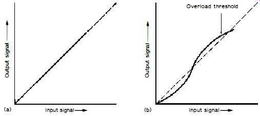
Fig. 2.5: Input/ output characteristics. (a) Perfect straight
line amplitude linearity and (b) non-linearity referred to the straight
line condition (shown by broken-line characteristic) . All amplifiers
are subject to a degree of non-linearity which causes harmonic and intermodulation
distortion, but the curvature within the dynamic range of a hi-fi amplifier
is very small. Hence the low distortion yield of such amplifiers. At
overload all amplifiers show severe non-linearity.
Examples from two signals of f1 = 60Hz and f2 = 7000 Hz are f1 +f2 = 7,060Hz, f2-f1 = 6,940Hz, f2-2fl = 6,880Hz, 2f2-2fl = 13,880Hz, f2-3f1 = 6,820Hz, etc.
One can well imagine the incredible number of intermodulation products, as they are called, which could arise from more than two frequencies (music signal, for example) passing through a non-linear amplifier!
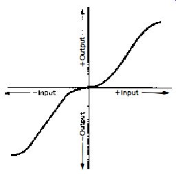
Fig. 2.6:
This sort of crossover non-linearity is responsible for crossover distortion
in some quasi-Class-B amplifiers (see text).
Crossover Distortion
The difference between simple harmonics and intermodulation products is that while the former are harmonious (musical instruments themselves produce harmonics which are responsible for the timbre of the sound) many of the latter are highly dissonant (having no acceptable musical relationship). However, a well designed amplifier of low THD should not generate much more IMD within its dynamic range; but like THD, the IMD will rise swiftly at the overload threshold. With some of the less detailed quasi-Class B amplifiers there is also the tendency for the distortion to rise at the low end of the dynamic range. This is caused by mild discontinuity of the input/output characteristics of the two push-pull output transistors at the crossover point, as shown exaggerated in Fig. 2.6. This reveals that at low output levels significant non-linearity occurs, also see (b) in Fig. 2.4.
The resulting crossover distortion is exposed more at low output by using an IMD test than a THD test, but not all specs give an IMD parameter at very low level. In the example spec it will be seen that the parameter relates down only to half rated power. Good test reports and reviews are sometimes more critical in this respect, so to get the full story on distortion performance they are well worth investigating.
IMD Spectrograms
The spectrograms in Fig. 2.7 show IMD products of two amplifiers from equal amplitude driving signals of 15 and 16kHz. No product is much greater
(a) (b)
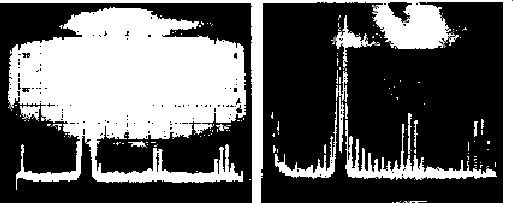
Fig. 2.7: Spectrograms showing IMD using twin tones (i.e., two driving
signals of equal amplitude), (a) low distortion amplifier and (b) amplifier
producing high distortion.
Scale 5kHz/ 10dB/div. than -70dB (0.03%) at (a), but at (b) there is a product up to -56dB (0.16%). Displays such as these given in test reports and reviews will indicate the voltage of each driving signal and the type of output load employed.
You should note in particular the amplitude and number of IMD products relative to the voltage of the driving signals and the type of load used, remembering that a loudspeaker type load can produce more distortion than a resistive load, especially at the top of the dynamic range where the phase angle of the load may be resulting in premature limiting of the amplifier, as already explained.
The spectrogram of a badly distorting amplifier with driving signals at about 100Hz and 1 ·4kHz is shown in Fig. 2.8. Notice here the large number of products and the large amplitudes of some of them.
In general, then, look for an amplifier with the lowest values of THD and IMD, but remember that an amplifier of relatively large THD may sound ...
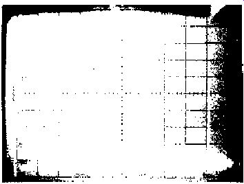
Fig. 2.8: Very bad I MD. Scale 2kHz/ 10dB/ div.
... better than one of smaller THD when the harmonics of the latter are dissonant . A better correlation between the measured results and the 'sounding' of an amplifier is given by IMD, particularly when expressed by a spectrogram (also see Section 9) . Power Bandwidth This refers to the frequency range over which a given output power can be obtained with respect to a specified level of distortion. A resistive load is employed and the distortion datum is usually 0.5 or 1 % . The more recent way is to refer the bandwidth to the rated power of the amplifier at 1kHz.
Thus, if the rated power at 1kHz is, say, 20+20W, then the power bandwidth refers to those frequencies below and above 1kHz where 20+20W can be obtained at a distortion no greater than, say, 1%, as shown in Fig. 2.9.
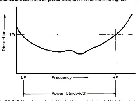
Fig. 2.9: Definition of power bandwidth. In this example the bandwidth
is from the low frequency ( LF) to high-frequency ( H F) points where the
distortion is 1% at the . amplifier's rated power.
The half power bandwidth refers to the low- and high-frequency points where the distortion is no greater than 0.5 or 1%, but this time at half the rated power of the amplifier . The bandwidth is greater from a given amplifier under these conditions than when the bandwidth is referred to the rated power . Although the 'energy' of music signal is less at the low and high frequencies than at mid-spectrum (music signal tends towards maximum at 700Hz) , it is desirable for the amplifier to be capable of delivering its full rated power without clipping and hence distorting down to at least 40Hz to at least 10kHz.
It is noteworthy that clipping distortion from amplifiers unable to deliver the rated power at low and high frequencies (including low power amplifiers) is a common cause of thermal damage to loudspeaker drive units.
Frequency Response
Whereas the power bandwidth refers to the frequency range at power, the frequency response is a lower level parameter, it indicating how the output varies over the frequency range at 1 W or less output.
A hi-fi amplifier should boast a virtually flat frequency response from at least 20Hz bass to 20kHz treble. The response is usually plotted in the form of a curve relative to 0-dB at 1kHz, as shown in Fig. 2.10. Here the output remains essentially constant from 20Hz to in excess of 20kHz; at 10Hz it is 5dB down and at 100,000Hz 10dB down! If 0-dB corresponds , say, to 1V across the output load, then at points where the response is - 5dB the voltage will be 0.562V and at -10dB it will be 0.316V. Based on power where 0-dB corresponds to 1W, say, at -5 dB the power will be 0 · 316W and at -10dB it will be -0.1 W. Half power corresponds to -3dB, as already noted elsewhere.
The decibel (dB) scale is thus a logarithmic scale of voltage or power ratios.
The dB scale is used in hi-fi because it correlates much more than a linear scale to the way that we hear . More details about the way that the dB is used in hi-fi can be obtained from the companion volumes Tuners and Amplifiers, Pickups and Loudspeakers, Improving Your Hi-Fi, ABC of Hi-Fi, Audio Technician's Bench Manual, etc.
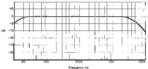
Fig. 2.10: Example frequency response which can be defined as 15Hz to
45kHz -3dB.
Half Power Point
The -3dB, half power point is significant in frequency responses, for some responses may be expressed as, for example, 10Hz -40kHz (-3dB) . This means that the frequency range lies between the points on the response where the output has fallen by 3dB ref. 0-dB at 1kHz. In Fig. 2.10 this would be between about 15Hz and about 45kHz. A plotted curve is better, though, since it shows unambiguously how the output rises and/or falls between the two -3dB points.
The frequency response is modified by the filters, loudness control, tone controls, etc. The accuracy of the RIAA equalization for the gramophone pickup is also shown by a frequency response. For this measurement an RIAA recording filter is connected in series with the test signal source.
Filters
Although the intrinsic frequency response should desirably be 'flat ' over the spectrum with minimal undulations, there are times when better reproduction can be obtained by deliberately reducing the output at certain frequencies.
One example of this is at the high-frequency end of the spectrum when reproducing program material which is rather 'noisy' - for example, from a scratched gramophone record or 'hissy ' FM stereo radio program.
By rolling-off (as it is called) the hi-frequency end of the spectrum the clicks from the record and the 'fizz' from the radio tuner can be reduced. This is because such disturbances contain components which extend well beyond the upper musical frequencies. However, if the roll-off is started too early the treble of the music will be diluted and the reproduction will lack the sparkle and attack associated with hi-fi.
When the unwanted noises are bad, a compromise between music quality and roll-off frequency has to be adopted, which is why some amplifiers allow you to switch the roll-off frequency. The frequency response in Fig. 2.11 shows two high-frequency roll-offs, one starting round 9kHz and the other round 20kHz. The latter affects the music quality far less than the former, but the former will reduce background hiss more than the latter.
The turnover frequency is that frequency where the response is 3dB below the response at 1kHz and the steepness of the roll-off slope is given as so many decibels per octave. The least slope is 6dB/octave, and this can catch some of the higher wanted music frequencies. The greater slope of 12dB/octave is generally preferable for filtering, for the turnover frequency can then be made higher with the swift fall blocking most of the noise components. Higher rates are sometimes used, but filters of this kind tend to impair the transients of the music, causing 'ringing ' and overshoot with a consequent tonal distortion on the reproduction.
In addition to turnover frequency switching, some amplifiers are also equipped with a control for varying the roll-off rate. Such filters, cutting the high frequencies, are known technically as low-pass filters because they pass the lower frequencies below the turnover frequency.
The filter at the other end of the spectrum is called a low-frequency, bass or high-pass filter. Except for large organs, there is not much in the way of music content below about 20Hz, so it can sometimes be undesirable for the amplifier to respond much below this frequency. Warps on gramophone records, for example, can produce sub-bass frequencies which merely cause the cone of the bass loudspeaker unit to pump in and out, thereby using up amplifier power unnecessarily and contributing to the distortion.
A bass filter round 20Hz turnover avoids these problems, while also reducing the lower frequency rumble of turntables. A higher turnover is needed, though, to eliminate all the rumble, particularly of a poor deck, and the roll-off rate must be greater than the minimal 6dB/ octave to prevent the wanted low bass music frequencies from being unduly attenuated. Responses of such filters are given in Fig. 2.12.
The parameters of filters may thus either be expressed by frequency/amplitude plots or by figures, such as 8kHz-3dB and 12dB/octave, 12kHz-3dB and 6dB/octave , 30Hz-3dB and 12dB/octave, etc.
Tone Controls
A tone control is really a filter of 6dB/octave maximum roll-off rate which is adjustable to give both cut and boost. It is also sometimes possible to switch the turnover frequency for a greater overall versatility of control. All hi-fi amplifiers have at least two tone controls, one for bass and the other for treble. Some have an additional control giving lift and cut round 1 or 2kHz.
Parameters may be expressed by frequency/amplitude plots as shown in Fig. 2.13, at (a) for un-switchable controls and (b) for two pairs of turnover frequencies, or by figures. Typical parameters for bass and treble are bass ± 1 0-dB at 100Hz and treble ± 1 0-dB at 10Khz. In Fig. 2.13 the middle sweep is with both controls at 'neutral' (flat), the top sweep with bass and treble and full lift and the lower sweep with bass and treble at full cut.
It can sometimes help to apply a little boost or perhaps cut at the bass or treble to improve the reproduction in relation to the program information or the acoustics of the listening room, including the loudspeakers; but in general excessive boost or cut is unnecessary.
Tone controls tend to provide an undesirably wide range of control. Tone controls can - and do -introduce distortion of various kinds, and because of this certain hi-fi freaks are tending to prefer amplifiers without such controls or, at least, with a switch to bypass the tone control stages.
Loudness
When the loudness switch is operated, the frequency response of the amplifier changes as the volume control is turned down to reduce the sound intensity.
What happens is that the middle of the spectrum becomes more attenuated than the bass or treble ends as the control is retarded, with the result that the bass frequencies, and to a smaller degree the treble ones, are boosted relative to the middle frequencies. This tends (unnaturally!) to compensate for the way that we hear. For "instance, as the sound intensity is reduced so the 'sensitivity' of our hearing falls at the bass and to a smaller extent at the treble.
Our sample spec shows that when the volume control is turned down from maximum so that the gain is reduced by 30dB (a thousand times power reduction) a boost of 8dB occurs at 100Hz and a boost of 4dB at 10kHz. The effect is revealed graphically in Fig. 2.14. The boost increases as the volume control is further turned down and decreases as it is advanced - but, normally, only when the loudness switch is on. With the switch off the volume control works normally without frequency compensation.
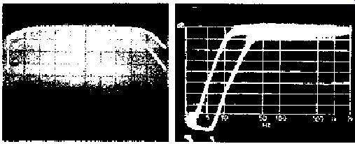
Fig. 2.11: (left) Frequency response showing two high-frequency roll-offs
and a smaller low-frequency roll-off. The high-frequency roll-offs correspond
to two, switchable low-pass filters. Scale 10dB/div. vertically and three
divisions per frequency decade horizontally, sweep logarithmic 20Hz -43kHz.
Fig. 2.12: (right) Bass filter (i.e., high-pass filter) response at two turnover frequencies. Scale 5dB/ div. vertically and Hz x 10 logarithmic sweep 20Hz -20kHz. (a) (b)
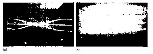
Fig. 2.13: Tone control responses, (a) fixed turnover frequencies and
(b) switched turnover frequencies, scale as Fig. 2.11.
Some amplifiers and receivers , though, notably European (not British) makes, are equipped with un-switchable loudness permanently 'ganged' to the volume control . This is not a particularly desirable attribute, but it is possible to counteract the effect by turning back (for cut) the bass and treble controls when listening at low level.
Damping Factor
When a loudspeaker receives from the amplifier a sudden pulse (e.g., music transient) the cone is swiftly deflected. After the transient has passed, the cone will return to its steady-state position. However, if the loudspeaker is inadequately 'damped' the cone will overshoot and move to and fro before finally coming to rest . This tends to 'color ' the reproduction, sometimes emphasizing 'bass boom' or 'one-note bass'. When the cone is vibrating due to lack of damping, the loudspeaker acts rather like a dynamo. Electricity flows out of the loudspeaker into the amplifier (an effect which can cause some amplifiers to produce interface intermodulation distortion - IID). If the output terminals of the amplifier 'look' like a very low resistance then the cone vibrations are quickly suppressed or damped. An amplifier with a high damping factor is endowed with a very low resistance output (just the matter of a few milliohms) and hence the loudspeaker is nicely damped.
The damping factor is numerically equal to the loudspeaker's impedance divided by the amplifier's output impedance. Thus with an 8-ohm loudspeaker, an amplifier with a source impedance of 0.1 ohm (100 milliohms) will have a damping factor of 80. It is important for the damping factor to remain reasonably high at very low frequencies for it is at the bass end when high damping is necessary to reduce the so-called 'one-note bass' effect of certain loudspeakers . The actual damping, of course, is always less than that provided by the amplifier because in series with this damping will appear the resistance of the loudspeaker's speech coil , frequency-divider components and loudspeaker connecting cables . It appears that there is little point in providing an amplifier damping factor greater than about 30 owing to these series effects . S/N Ratio While the maximum output of an amplifier determines the top end of the dynamic range, the lower end depends on how much noise the amplifier is producing. If the noise is relatively high, then very quiet parts of the music will be masked and there will be a loss of information. The noise is measured, often through a 'weighting' filter which simulates the way that we actually discern the noise (see Section 3), relative to the amplifier's full output . It thus gives an expression of dynamic range.
Ratios of 66dB phono (magnetic pickup) , 70dB auxiliary and 75dB tape are perfectly acceptable. The measurements are made with the appropriate input loaded and with the volume control at maximum. Under normal music conditions better ratios generally occur because we rarely operate with the volume control flat out !
Residual Hum and Noise
This measurement is similar to S/N ratio but it is made with the volume control turned right down so that it is the hum and noise of the stages after the volume control which in this case are evaluated. The actual hum and noise voltage across the amplifier's output load is commonly measured which, in the sample spec, is lm V. This corresponds to the mini-power of 1.25 x 10^7 W, so you would have to get very close to the loudspeaker to hear the result!
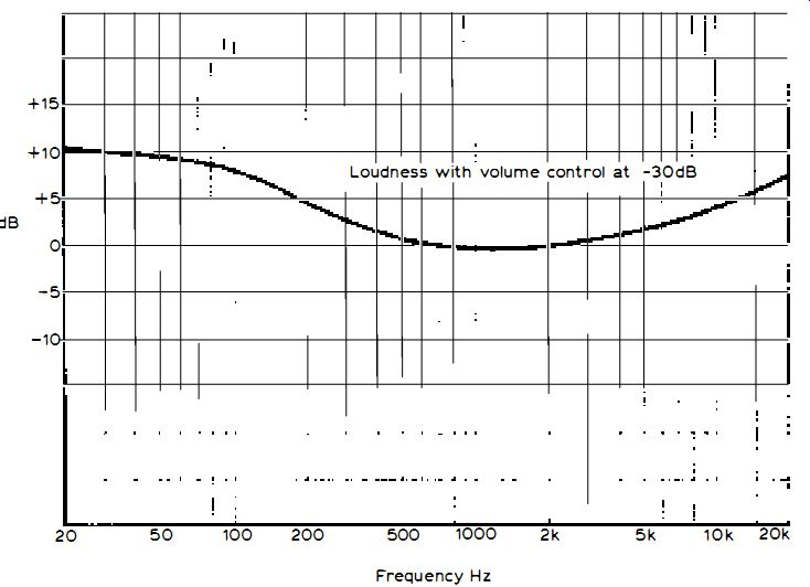
Fig. 2.14: Loudness response with volume control set at -30dB.
Input Sensitivity and Impedance
This parameter tells you the level of signal at mid-spectrum (1 kHz) that the amplifier needs at any of its inputs to give its full output with the volume control at maximum (all other controls at 'neutral' or switched out) . It also tells you the impedance or resistance that the inputs present to the program sources . The particular program source should give an 'average' signal fairly close to the appropriate input sensitivity and the impedance or resistance reflected from the input should not adversely affect the signal from the source . In the latter respect , it is best for the impedance or resistance of the input to be greater than that of the source. The frequency response of the source is then affected least . The other way round, the capacitances of the screened signal-coupling cables can cause high-frequency roll-off of the source signals.
The absolute performance of a magnetic pickup (cartridge) is often determined by the 'load' it 'sees ' from the phono (pickup) input . The average cartridge load is round 47k-ohm, which is why the pickup input impedance is close to this value. However, this is less applicable to low impedance cartridges , such as moving-coil types . On the other hand, certain relatively high impedance cartridges are very critical to load, including shunt resistance and capacitance, and some of the better class amplifiers and hi-fi receivers cater for this by input impedance switching.
In general, the input sensitivities and impedances of latter-day amplifiers and hi-fi receivers are carefully tailored to suit current signal sources so there should not be too much trouble in securing a fair coupling match, and they are switchable on some amplifiers.
Pickup Overload
Although the 'average' output of a pickup may only be some 5mV, to give the full dynamic range of the record the signal level will vary over some 60dB relative to this 'average'. At very low outputs the overall noise becomes significant, while at very high outputs the distortion and overload take effect.
Thus to avoid serious distortion at high outputs the RIAA preamplifier must be capable of handling the signal without overloading. This is expressed at 1kHz by the pickup overload parameter.
In the sample spec it will be seen that although the input sensitivity at pickup is 2.5mV, the input will accommodate up to 100m V before serious overload becomes apparent . These are r.m.s. values . Peak values (that is the r.m.s. value times 1.414) are more meaningful here because the recording level of records is given in terms of peak velocity.
Peak recording levels up to at least 30cm/sec. can be detected, so if the pickup has an output of, say, 1.5mV per cm/S. recording level, then the peak output can be as high as 45mV (corresponding to about 32mV r.m.s. on a sinewave basis) . To be on the safe side a 6dB (2 times voltage ratio) margin should be allowed, thereby bringing the figure up to 64mV r.m.s. equivalent.
The sample spec shows that this is well catered for since the overload threshold is as high as 100m V r.m.s. for 0.5 % distortion level . Pickup pre-amplifier overload cannot be eliminated by turning the volume control down because the volume control appears at its output . Pickup overload, therefore, can be responsible for poor reproduction even when playing at moderate sound levels. The effect is not unlike pickup mistracking.
The overload margin commonly deteriorates with reducing frequency, which is another reason why a 6dB margin should be allowed. At frequencies above 1kHz the margin widens due to the action of the RIAA-equalization on the preamplifier's feedback, but , then, at these higher frequencies the pickup output can be greater anyway! Tape Recording Output This is the signal output delivered by the tape recording outputs of the amplifier or hi-fi receiver. It is commonly independent of the volume control setting, tone controls and filters but dependent, of course, on the level of the source signal . At the 'phono' output sockets the signal level is round 150-200mV 'average', which suits the majority of tape machines with this sort of recording input socket . The recording output to the DIN socket is less than this , for DIN-based tape machines call for a much smaller signal for full recording level . The DIN 'constant current' recording standard is nominally 1-mV for each 1 k-ohm of load resistance presented by the tape machine - so if the recording input load of the tape machine is, say, 47k-ohm , then the signal across the DIN socket will be round 47m V 'average'. Other Parameters These, then, are the 'standard' engineering parameters that accompany an amplifier or the amplifier section of a hi-fi receiver (formerly called tuner amplifier) . They do let you know how powerful the amplifier is, how well it has been designed, whether it is worth its money, etc. They do not, however, let you know exactly how the amplifier will audition to the listening room.
In addition to the basic engineering parameters other factors are here involved, including the quality of the signal sources and loudspeakers, how well the loudspeakers interface the amplifier and various other objective/subjective parameters which are only recently being brought to light . Some of these are considered in Section 9.
You must be able to judge the engineering parameters, nevertheless, to discover whether the amplifier is powerful enough for your requirements, whether it will satisfactorily match the signal sources , whether the tone control and filter characteristics are to your liking, etc.
It is sad that amplifiers are judged in terms of watts of power output . Signal voltage output across specified load conditions would be far more appropriate. This is because the sound pressure level (SPL) produced by a loudspeaker is generally rated in terms of signal voltage across it . A loudspeaker spec may include the parameter of 96dB SPL for 6V input measured under anechoic conditions (e.g., non-reverberant room) at 1 m.
In a normal domestic situation you will be using two loudspeakers for stereo, the room will be reverberant, depending on its size and furnishings, and you will not be sitting at lm from the loudspeakers. In an 'average' listening room at normal listening distance from the loudspeaker 96dB SPL will be evoked when the signal voltage to each loudspeaker is a little over 2 times that of the exampled loudspeaker parameter . In other words, each loudspeaker will require an input of about 13V. If the loudspeakers each have a nominal 8-ohm impedance (equivalent resistance) , then to produce 13V across each one, each channel of the amplifier will have to be rated round 21 W. This applies to a typical lounge size of some 703m. An SPL of 96dB is remarkably 'loud', and under most normal conditions you would generally be peaking below this . You will have to make sure your amplifier choice provides this sort of output at low distortion.
= = = =