Are intermodulation distortion figures far more relevant
than those of THD in measuring amplifier sound quality ? This author,
with his explanation of what IMD is and how to measure it, believes so.
By Anthony New
(Reprinted with permission from Electronics World.) Although IMD has not been discussed as much in the design of audio amplifiers compared with THD, there is consider able literature on IMD in general and its application to RF amplifiers. For this reason, I will give a simple overview of IMD and point out a few implications for its use in audio design.
WHAT IS IMD?
In general, IMD is produced whenever two or more signals with distinct frequencies F1 and F2 pass through a device-be it an amplifier, filter, or other circuit-that possesses an amplitude nonlinearity of the form:
Y = A1X + A2X2 + A3X3 +A4X4 + A5X5 +
... where A1 is the nominal gain of the amplifier and the higher powers of X correspond to the various nonlinearities that may be present. I have ignored phase nonlinearities here for simplicity.
This nonlinearity produces IMD products at the following frequencies ...
nF1 + mF2
...where n and m are non-zero integers.
Note that if you put n.m = 0, you get purely harmonic distortion rather than IMD, which indicates that harmonic distortion is a special case of a more general phenomenon.
The order of the IMD products is de fined as:
k = ?n ?+ ?m ?
.... so that the "third-order" products that often dominate are of the form:
F1 ± 2 × F2, F2 ± 2 × F1 and 3 × F1, 3 × F2
In RF amplifiers a further restriction often applies. Even in many "wideband" products the overall bandwidth of the amplifier is less than an octave, and so only those odd-order products with ...
?n ?- ?m ?= ±1 ... are "in-band" and of concern.
Consequently, even-order nonlinearities--second, fourth, and so on-which produce no odd-order products are usually ignored.
However, in a multi-octave device such as an audio amplifier, this restriction will not apply. The most common and usually most important non linearity is, however, still a third order nonlinearity of the form:
Y = A0X + A3X3 which will result in IMD products of third order only, namely (2F1 - F2, 2F2 - F1, 2F1 + F2, and 2F2 + F1).
The first two represent the classical IMD products and the other two are higher-frequency IMD products, at roughly three times the fundamental frequencies when these are close together.
The spectrum of Fig. 6 in Part 1 shows these third-order products of a two-tone signal, in addition to higher level, second-order products. Note that only the third-order products are close in frequency to the input tones.
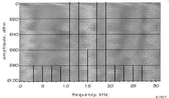
FIGURE 7: Idealized spectrum of four-tone test sometimes used with RF
amplifiers. The four main tones are harmonically related, phase-locked
and phase-peaked to maximize the peak value of the signal envelope in
the time domain. This-in an RF amplifier, at least-is likely to maximize
the visible third-order IMD products, particularly the central one between
the two pairs of tones which thus makes an easy frequency component to
check. With zero IMD this component would be completely absent.
Figure 7 shows an idealized spectrum of four-tone test sometimes used with RF amplifiers. If the power input to the device is varied, the output levels of the IMD products will vary, too. This is shown in Fig. 8, from which you can see that if the input level increases by 10dB, the third-order IMD products increase in absolute level by 30dB. Their level relative to the wanted output signals also increases by 20dB. If the straight lines are extended to the right, you will see that they all meet at a single point. For obvious reasons, this is known as the "output intercept point." Strictly in this instance, it is the "two-tone, third-order output IMD intercept point," or IP3.
For any signal below this point, you can estimate the level of IMD products by subtracting the output signal level from the IP3 to give a figure in decibels, and doubling this to give a figure in dBc. This represents the IMD relative to the "carrier," i.e., wanted signals, assuming them to be similar in level.
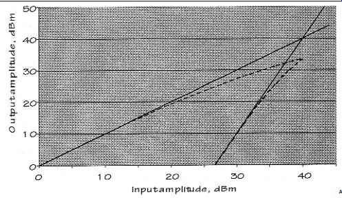
FIGURE 8: Amplitude response of amplifier displaying "classical" third-order
IMD. Amplifier input signal level is displayed on the X-axis, and output
level on the Y-axis; both axes are logarithmic. The straight line through
the origin represents ideal linear response. The straight line at a steeper
angle shows the theoretical level of IMD products, which change three
times as quickly with input amplitude as the signal itself. The point
where the straight lines meet is the IP3. The curved lines show the likely
real characteristics as the amplifier begins to clip. However, for sensible
operating points well below the IP3, the straight lines are a fairly
good match for a single-stage class-A RF amplifier without any special
linearization techniques. The IP3 concept is also useful for other devices
such as mixers, which also display IMD. For any input signal level on
the X-axis, the upper line will show the nominal output level, and the
vertical separation between the two straight lines will show the expected
linearity in dBc. When high-level multi-tone signals are concerned, this
figure-rather than the noise figure-usually rep resents the dynamic range
of the signal, since it indicates the relative level of interfering products.
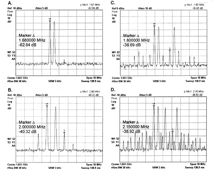
FIGURE
9: Spectrograms of real signals. For convenience these have been taken
at RF, though similar spectra could be observed at audio. (a) two-tone
signal, no visible distortion; (b) two-tone signal plus obvious third-order
IMD; (c) three-tone signal; and (d) four-tone signal. Note that each
extra main tone produces many extra IMD products. In (d) the tone frequencies
have been deliberately chosen to make as many products visible as possible;
usually sever al would either overlap or appear to do so within the resolution
of the spectrum analyzer. However, in a complex musical signal the large
number of signal tones would cause the hundreds of IMD products to merge
into a noise-like background which reduces the clarity of the signal.
REAL SIGNALS
It is highly unlikely that a real device could be operated anywhere near its IP3 point, which is only useful for calculation and reference. Also, a real device is likely to show IMD at other orders, particularly fifth, when it is driven at all hard. As these will reduce by the fifth power of the signal level instead of the third, though, they are likely to be lower in level. However, a fifth-order nonlinearity will also produce some third-order IMD.
This may even cancel out some or all of the third-order IMD produced by the third-order nonlinearity, resulting in the fifth-order IMD product dominating at some output power. A similar situation exists for higher-order IMD products, but the actual levels are generally both lower than third- and fifth-order IMD products and rather less predictable.
When more than two large signals are sent through the same amplifier at the same time, the number of IMD products grows rapidly. Figure 9 shows spectra of a real, albeit RF, amplifier with real multi-tone signals.
Two tones produce two close-in IMD products, in addition to the other distant ones shown in Fig. 6, but nine products are visible with three tones (Fig. 9c).
With four tones the number increases again (Fig. 9d), though in practice some of these may be co-incident.
When a complex modulated signal is used rather than a set of CW tones, the IMD products occupy a bandwidth rather like a noise spectrum.
Since these IMD products are not harmonically related to their causative signals, they behave like noise, too, reducing the intelligibility of speech or data transmissions to a measurable degree. It is not possible to filter them out, since although the bandwidth they occupy increases with their order of distortion (Fig. 10), their bandwidth always includes the original signal.
MEASURING
As I commented, one of the benefits of IMD over THD is the relative ease of measurement due to the distorted products being not harmonically related to the original signals. A typical setup will consist of a pair of signal generators- or, often, a dual-output generator-a linear combiner, possibly resistive, and a spectrum analyzer (Fig. 4 in part 1). The analyzer display will then look some thing like Fig. 6 if the analyzer span is sufficiently wide, or like Fig. 9b in the more usual narrowband case.
The IMD products may be much lower in level, but are easily seen, provided the analyzer has enough dynamic range. If the analyzer has appropriate delta markers, you can simply read the relative distortion off the screen display. If not, a little mental arithmetic is required.
Note that with IMD tests it is not necessary to use especially low-distortion oscillators, since the harmonics produced will not normally interfere with the measurement process. However, the linearity of commercial spectrum analyzers is rarely much better than 80dBc-or 0.01% in voltage terms-and may be poorer. For the best amplifiers some additional filtering may be needed to notch out the pure signals, or a coherent subtraction method (Fig. 5).
Another test commonly used is the four-tone test illustrated in Fig. 7. Here, four tones at, say, 3, 4, 6, and 7kHz are produced by four phase-locked generators and the analyzer tuned to look for the missing 5kHz component, which can only arise from a nonlinearity.
FIGURE-OF-MERIT
A figure-of-merit commonly used in RF amplifier design is the intercept point in dBm (Fig. 8). The higher this is for a given power level required from the amplifier, the lower will be the distortion produced, and from this IP3 figure it is quite easy to calculate how much distortion is likely at any given power level.
However, at this point I should comment that one of the many differences between RF and audio amplifiers is that RF amplifiers are usually operated somewhere near their continuous peak power rating. Alternatively, they are at least backed off from this by a consistent amount. Also, they do not often use feedback to achieve good linearity. Consequently, they may have an IMD response which approximates to a classical curve over most of their useful power range and for which a single IP3 specification is a useful measure of linearity in any application.
Where real audio amplifiers are concerned, I believe that typical responses are unlikely to be so simple over the wider range of signal levels encountered, particularly in a "blameless amplifier," where all of the distortion mechanisms have been separately identified and reduced to a low level by various means. Furthermore, audio music signals can have a very high peak-to mean ratio. It is common practice to specify amplifiers with a power handling greatly in excess of what is normally required. As a result, much of the time they will be operating at a very small fraction of their nominal power output, where the real distortion produced is somewhat different from the "classical" third-order model.
It is likely, therefore, that rather than a single calculated IP3 figure, a curve of measured IMD levels versus signal level is more appropriate, rather like the waterfall spectrographs sometimes used. It would also give a far better indication of the order of distortion produced than a single figure, even an IP3 figure.
Nevertheless, the level of intermodulation produced by an amplifier is, as I have shown, absolutely critical to its quality as an audio device. Any useful specification for its linearity should reference this. I therefore propose that the specification should be something like this: "Two-tone third-order IMD performance: better than -70dBc over 0.1W to 30W and 50Hz to 20kHz" or something similar. In practice, it may be necessary to limit the tests to a set of standard test tones, for example, 3.5kHz and 4.5kHz. Intermodulation products would be looked for at 1kHz, 2.5, 5.5, 11.5, and 12.5kHz.
Harmonic products at 7kHz and 9kHz might also be present but could be due to the signals sources themselves. It would also be possible to re peat the test at additional low and high frequencies to test IMD performance there, such as 350/450Hz and 15/16kHz.
Of course, modern lab equipment is capable of performing swept measurements and downloading the results to a PC for analysis and printing, so a swept measurement may be acceptable as a standard.
SECOND-ORDER NON-LINEARITY
The third-order function discussed earlier was selected to represent a typical amplifier nonlinearity. What would happen with an amplifier having a second-order nonlinearity ? This is a rather interesting case study, as it helps to explain the difference between "valve sound" and "transistor sound," which used to convey such emotion many years agoand in some circles still does.
A second-order nonlinearity such as that often found in a thermionic valve produces second-harmonic distortion- which is not unpleasant in moderation.
And it produces only even-order IMD, namely zeroth and second-order, at low level. It produces no odd-order IMD products of the form (F1 ± 2 × F2). A narrowband amplifier produces no in-band IMD at all. Thus the absence of any second-harmonic cancellation in a class-A configuration has no impact on the IMD present, as suspected by those who prefer this configuration.
For much of the music program, the loudest frequencies present in the signal will often be harmonically related.
Many of these extra distortion terms, of the form F1 ± F2, will fall on, or close to, existing signal frequencies at much higher level and may be reasonably effectively masked.
Provided the levels of distortion are not excessive, the result will probably not be particularly unpleasant, and may give the effect of a warm coloration to which you can become accustomed. Note that this form of distortion reduces markedly as output level drops, so that soft passages may be portrayed quite realistically. Loud passages are likely, in any case, to have a richer harmonic texture which hides the IMD more effectively.
In contrast, the chief distortion mechanism of early transistor amplifiers was not large-signal output device nonlinearity, but crossover distortion.
This generally becomes increasingly noticeable at low volume settings.
Large amounts of feedback were often added to cure this and other problems, though the designers perhaps did not always appreciate how much the loop gain dropped in the crossover region.
Consequently, transistor amplifiers tended to suffer from less high-amplitude low-order nonlinearity and more low-amplitude high-order distortion.
The effect of this on the reproduced sound was quite distinctive. Gone was the warm colored but fairly clean sound familiar to many who hadn't perhaps experienced the best valve amplifiers.
Even by the 1960s, these could boast less than 0.1% THD, most of that being the relatively benign low orders. In its place was a cold, muzzy (and some times hissy, but that's another issue) sound that could be particularly noticeable in solo piano works. I think the worst commercial design I ever heard was the "Sinclair 2000," which was pretty, but built down to a price.
It has been said that the unthinking application of negative feedback around an amplifier can often merely transform large amounts of low-order distortion into small amounts of high order distortion. It is also true that any crossover-induced IMD remaining after the application of negative feedback is still present at low signal levels rather than diminishing with volume.
It would have been nice had designers appreciated the futility of their policy of measuring distortion in terms of THD at full output. Instead they concentrated in reducing it, albeit with some success. To those concerned with measurable THD, the trade-off seems worthwhile, but the high-order IMD products were usually spread far away in frequency from any masking tones in the signal, and were thus very audible.
On complex music containing many strong frequency components, the large number of high-order products degenerate into a background noise. This noise is signal-dependent and hides any subtle details from the ear (Fig. 10). It is no accident that the "clarity," often regarded as the highest accolade in audio, is the direct result of an absence of IM products.
TIM AND OTHER FACTORS
Distortion in phase can also occur in an amplifier that causes changes in pulse response. Real amplifiers also usually display some amplitude-to pulse modulation and pulse-to-amplitude modulation conversion, too. I have deliberately avoided discussion of these since there is considerable doubt whether modest phase effects are audible at all. However, it is less contentious to say that over some of the audible range at least, differences in phase response between channels will at the very least degrade or alter the stereo image presentation and are therefore undesirable.
There is another form of intermodulation distortion that has been discussed in audio design, namely, transient IMD, or TIM. This is the distortion said to occur when a part of an amplifier suffers slew-rate limiting. For a brief period of time, the amplifier is unable to follow the input signal at all. During this time the amplifier gain is zero.
The usual remedy is to ensure effective low-pass filtering prior to any stage that suffers slew-rate limiting. But since the event is transitory, the distortion may not show up in steady-state measurements-particularly the continuous-sine waveforms generally used in total-harmonic distortion measurements. With a suitable input signal, though (one with a high peak-to-mean ratio, perhaps), this should show up in an intermodulation distortion test.
Other test waveforms are often used with amplifiers; for example, square waves to show load stability. These may well continue to be necessary, though it may be sufficient-and perhaps prefer able-instead to measure the IMD performance with a range of realistic load impedances, since it is the distortion we are primarily interested in.
SUMMARY
I have shown here that current testing methodology fails to test the performance of audio amplifiers adequately in a manner that relates to audible performance. It fails to measure what it purports to do, namely, the difference between a representative complex and time-varying signal input to an amplifier and the actual output from it.
Instead, testing concentrates on an extremely narrow interpretation of "distortion" that the ear doesn't actually hear as distortion at all. It makes no at tempt to measure important types of distortion that certainly are audible.
And it does not apply the same rigor to frequency-response issues that it does to THD. Tests for load stability are also generally done separately to other tests. This is presumably done on the assumption that variations in loads can't possibly affect other aspects! In my view, any real test of an amplifier should apply a representative complex signal and compare this with the actual output of the amplifier under a range of likely loads. This could be done in many ways, with real or artificial sources and measured over frequency or time.
A suitable and relatively simple means exists which is already used in other fields, namely, IMD measurement under multi-tone conditions. The exact format of these tests could, and should, be adjusted to maximize their relevance to the particular case of wideband ultra low distortion audio amplifiers. These or other measurements should also be capable of measuring frequency response to a far greater level of accuracy than is current.
When appropriate and psychoacoustically relevant tests are available, then perhaps we can better assess audio amplifiers objectively and better relate their objective performance to subjective tests.
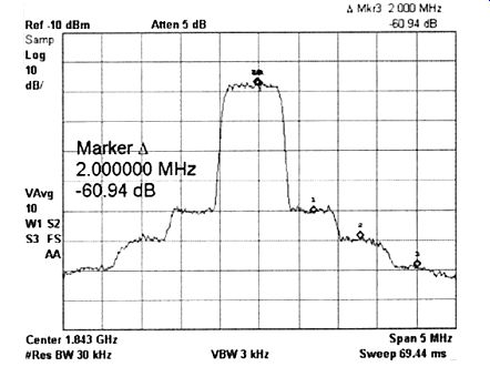
FIGURE 10: Example of a real modulated signal with IMD-here the IMD
products are not discernible individually but serve effectively to raise
the noise level in steps-each step corresponds to a particular order
of IMD. The first step on each side is produced by third-order IMD, the
next by 5th, the next by 7th, and so on. Note that the IMD products occupy
more bandwidth than the original signals; the higher the order, the more
bandwidth occupied. The step pattern might, however, not be visible with
the less-ordered spectrum of a typical music signal.
------------------
DECIBELS, DBM, DBW, AND DBC
It is common to specify amplifier distortion in terms of percentage, with the understanding that voltage ratios are intended. However, where loudspeakers have to be driven, it is power that is more relevant.
For constant-impedance systems with a wide signal range, a convenient logarithmic measure is the decibel, or dB. This is strictly a ratio of two quantities with the convenient feature that 10dB corresponds to an increase in signal power by a factor of ten, and 20dB corresponds to an increase of ten in voltage and ten in current, making 100 in power.
Specifying an increase of 20dB is then unambiguous, regardless of whether the speaker is thinking in terms of power or voltage.
Where an absolute level is needed, the terms dBm, i.e., dB relative to one milliwatt, and dBW, i.e., relative to 1 watt, are commonly used. In specifying levels of distortion, a further measure is useful, namely dBc. This refers not to a noise-suppression scheme but to decibels relative to the carrier, i.e., the main signal.
Where multi-tone signals are present, there is, however, a further possible confusion between dBm/tone, dBm mean, and dBm peak.
-AN
----------------------
Also see:
Link | --Link | --A MODULAR HYBRID AMP SYSTEM
POWER TRANSFORMERS FOR AUDIO EQUIPMENT--Keeping the magnetic field where it belongs-out of the audio path. By Pete Millett