|
|
This highpass/bandpass/low-pass filter has a tunable fo (20Hz-20kHz) and a wide Q range (0.5- 00) for audio filtering, resonant tone pulse generation, auditory music analysis, measurements, and more.
The Sound Strobe generates six selectable-spectrum (but wideband) pulses that are very revealing of speaker transient precision and in-room sound clarity. The tunable, variable resonance filter I describe here allows focusing the pulses’ spectrum into a bandwidth (BW) ranging from 2.5 octaves to less than 1/48 octave (1/4 semi tone). Then, with octave switching or a 20Hz - 20kHz sweep control of fo, you can hear transient response, frequency response smoothness, image focus, and room acoustics effects, as a function of frequency. (fo is the bandpass output’s center frequency.)
With high Q (resonance) settings, the Sound Strobe pulses produce, at the bandpass (BP) output, an exponentially-decaying sinusoidal tone burst, at the filter’s fo. These start with a clean and precise onset, producing a sound that resembles musical tone transients. Be cause of this, you hear the characteristics of speakers and room colorations with recognizable correlation to musical re production quality.
“AUTO Q” MODE
In addition to a manual mode (where you can adjust Q from 0.5 to 30), there’s an “Auto” mode. Here, the Q increases with the fo setting, ranging from 7.3 at 20Hz to over 100 at 20k.Hz. Used with the Sound Strobe’s “25ms exponential” pulse (a full-band step pulse rolled off below 6Hz), the filter’s BP output has sufficient resonant decay time to hear a distinct tonality, while being short enough to hear transient-response de tails. As you tune fo, the pulse sound has these characteristics:
1. fo range of 20-50Hz: resembles bass drums of various sizes.
2. 40-300Hz: the fundamental tones of a plucked string bass.
3. 300Hz-1kHz: chimes and bell transients, somewhat guitar-like.
4. 1kHz-3kHz: the metallic transients of small bells, xylophones.
5. Above 3kHz: high-pitched transients such as small triangles.
As you tune fo over the full audio band, a multitude of speaker and room anomalies can be revealed. Also, slowly sweeping fo allows you to hear the sound system’s coherence and smoothness (or lack thereof) of frequency response. And, as with the raw Sound Strobe pulses, you can easily discriminate the direct speaker sound from room effects. But with this filter, you can “hone in” on any specific frequency.
A switchable +1.82dB/octave slope equalizer (EQ, when used with the Sound Strobe 25ms exponential pulse and the filter’s “Auto” Q mode. maintains a constant energy per pulse regard less of fo.
These precise-transient exponential tone bursts, as their fo is swept, will reveal many details regarding overall speaker sound clarity timing precision, and spatial image focus.
OTHER FILTER USES
1. Auditory spectral analysis: Playing music through the filter (BP output) can be informative in several ways. With the Q(manual mode) set to about 4, the -3dB BW is about 1/3 octave (4.31 is the exact Q value). This is useful to explore the frequency range of various musical sources; with higher Q settings you can select individual instrument tone harmonics.
But perhaps the greatest use is in identifying the frequency ranges where there’s some coloration or distortion that you’ve previously noticed. For this purpose, it’s useful to feed one of the stereo channels through the filter, so you can tune the fo while also hearing the full-band sound from the other channel.
2. You can use the highpass (HP) and low-pass (LP) outputs with music to hear the effects of bandwidth restriction, and to determine the bass depth and HF extension in a particular piece of music. You should set the Q to 0.7, because this produces a Butterworth rolloff (maximally flat without peaking) of 12dB/octave.
3. Noise measurements: The HP and LP filtering can be useful in determining the noise voltage above or below some chosen frequency. The HP output is also useful to attenuate AC line hum.
4. Notch filter: A notch (about 40dB deep) response is easily generated by summing the LP and HP outputs with two 1k resistors. A low Q produces a wide notch, and higher Q values make the notch narrower. The passband voltage gain will be 0.5.
5. Any general-purpose applications where tunable filtering is needed.
6. Spectrum analysis: You can use the BP output with an AC voltmeter to measure audio waveform levels in tunable frequency bands.
7. Crossover design: Using the LP and HP outputs, with one inverted and Q set to 0.5, lets you experiment with CO frequency with a tunable second-order CO.
STATE VARIABLE FILTER BACKGROUND
In 1971, while working at APP Instruments (where I designed the APP 2600 synthesizer, made known by Stevie Wonder), I presented a paper at the Audio Engineering Society on “The Electrical Design and Musical Applications of a Voltage-Controlled Filter/Resonator.” The circuit I designed became the APP Module 1047 Multimode Filter/Resonator (Photo 1). This made the variable tonality effect in the rhythmic background of The Who song entitled “Won’t Get Fooled Again.”
Fast-forward 36 years: Photos 2 and 3 show the prototype of the circuit de scribed in this article. I haven’t designed it into an enclosure yet; I’m waiting to see whether there’s enough interest. See Fig. 12 for a recommended control component layout.

PHOTO 1: ARP Module 1047 (from 1971).
TOPOLOGY, FREQUENCY, AND SQUARE WAVE RESPONSES
The topology and Laplace (frequency domain) analysis of the state-variable filter (also known as the “Bi-quad”) are shown in Fig. 1. Figure 2 shows the frequency responses on dB versus log frequency scales. The principal advantages of this topology are (1) you can obtain a very high Q (up to 1000) with stability, (2) the latter doesn’t depend upon precise component value matching, and (3) you can achieve a very wide fo sweep range (over 1000:1) while maintaining response - shapes and unity-gain passband regions.
In Fig. 1, the elements labeled “-a” and “b” can be voltage controlled attenuators (VCAs) as in the design. The “a” elements must track, but can be either both inverting or both non-inverting. Inverting “a” elements provide non-inverting BP and LP outputs. Using a dual log pot for the a elements can provide about a 100:1 fo sweep, and both “a” and “b” can be fixed resistors for fixed fo and Q applications.
Figure 3 shows all three outputs’ responses to a 1kHz square wave, with Q values of 0.5 (non-resonant, left column) and 1.0 (slightly resonant, right column). Filter fo is set to 5kHz. The LP output is DC coupled, and at fo all three outputs have a voltage gain that’s numerically (not dB) equal to Q.
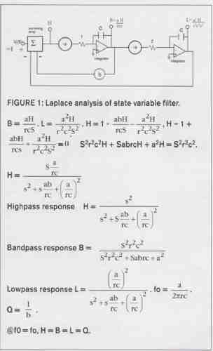
FIGURE 1: Laplace analysis of state variable filter.
Highpass response H =
Bandpass response B =
Low pass response L=
FILTER RESPONSES TO SOUND STROBE “PINK PULSE”
The “pink pulse” (Fig. 4) is so-called because, like pink noise, its spectrum is flat on a per-octave, per third octave (and so on) basis. The filter’s BP response, for a given Q also maintains a constant number of octaves (or fraction thereof) bandwidth regardless of fo. Therefore, the BP output from a pink pulse will maintain a constant energy per pulse as fo is changed. But with a constant Q setting, the pulse decay time is inversely proportional to fo.

Photo 2: New Filter Prototype.

FIGURE 2: Frequency responses of multimode filter.
To maintain constant pulse energy versus fo, the peak output voltage will increase proportionally to the square root of fo. With a step pulse filter input, the peak output voltage is constant with fo, so the decreasing decay time versus fo causes the pulse energy to decrease, inversely proportional to SQR-ROOT (fo); that is, at -3dB/octave. But this is expected, because the spectrum of a step pulse, while down-sloping at -6dB/octave on a per-Hz analyzed basis, has a -3dB/octave downslope on a per-octave basis. The latter, as explained in the Sound Strobe article, is the way we hear: we analyze spectra on a per-octave (or fraction) basis.
SOUND STROBE PULSE WITH HIGH-Q RESONANCE
In Fig. 4, the Q is a high value of 59, with fo = 5khz. Note the long resonant decay in the left waveform of Fig. 4B. The sinusoidal decay is a pure exponential; that is, a constant number of dB per time unit (linear dB/ms slope). This waveform takes 4.32ms to decay 10dB, and 25.9ms (130 waveform cycles) to decay 60dB.
This waveform is useful for hearing room acoustics properties; it’s resonant enough to produce a distinct tonality (the spectral BW is 0.0245 octave, or 0.391 semitone), but the 60dB decay time of 25.9ms is much shorter than the reverberation time of any room except an anechoic chamber.
The right photo in Fig. 4B is the same waveform expanded to a 0. time scale. Note the clean attack transient starting at the sinusoidal zero-voltage point. (The slight starting curvature is from the input pink pulse’s finite rise time of about l
TRANSIENT SOUND VARIATIONS
The resonant tone decay is the same at all three filter outputs (except for the +90° HP and —90° LP phase shifts regarding the BP out). But the transient “impact” sounds are quite different. The HP output (Fig. 4A) passes the frill HF content of the pulse, resulting in a much sharper transient sound (at the 5kHz fo shown, the sound starts with a metallic “ting”).
Conversely, the LP output transient is relatively “muted,” but with significant LF content (manifested in Fig. 4C by the first half-cycle of higher amplitude than the others).
Figure 5 shows the most extreme range of HF and LF transient spectrum emphasis available. In Fig. 5A, the Sound Strobe impulse waveform is used with the filter’s HP output. The impulse spectrum (flat per-Hz but upsloping +3dB/octave on the ear’s per-octave analysis) has its strong HF content passed unattenuated by the HP output.
Figure 5B shows the opposite available extreme: The Sound Strobe’s 252ps exponential pulse is used. This is a step pulse rolled off at 6dB/octave below 632Hz. The longer pulses (830us and 2 exponential) have more extended LF spectra, but I used the 252us pulse here so its decay could be seen on the fast (0.1ms/div) time scale. The LP filter output is shown; note the strong LF content as the resonant sine cycles have an initial offset that follows the input pulse decay. This type of waveform is useful for hearing a speaker’s full-band transient coherence in the presence of a tunable, musical-sounding HF resonant decaying tone.

FIGURE 3:1kHz square wave responses. fo = 5kHz, Q = 0.5 and 1. 1V/div, 0.2mS/div.

FIGURE 4
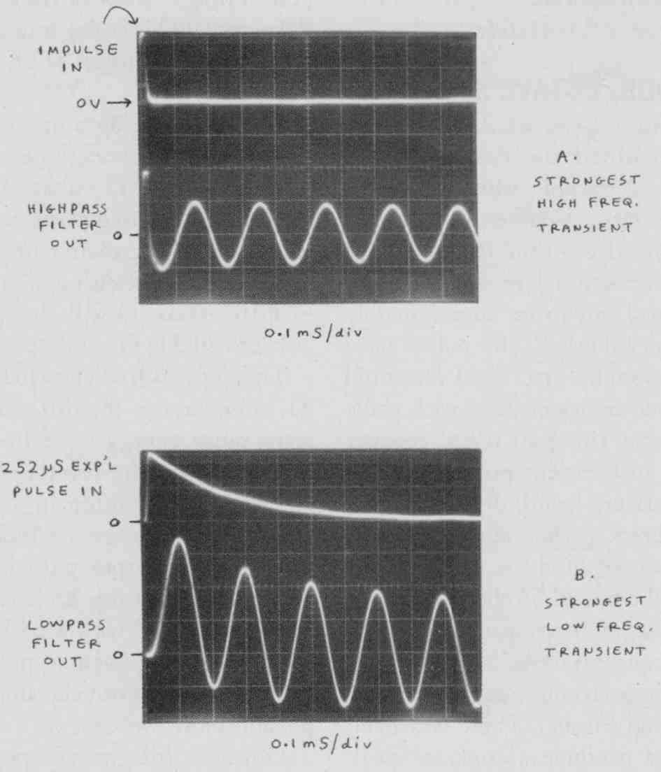
FIGURE 5: Sound Strobe pulse/filter combinations for strong HF and LF transients
at start of resonant tone decay. Fitter fo = 5kHz, Q = 59; 1V/div.
GENERAL PROPERTIES OF FILTERED TRANSIENT PULSES
Figure 6 shows a pink pulse through the BP output, with fo = 1kHz and a Q of 4.3 18, which corresponds (with a BP filter having ±6dB/octave asymptotic slopes) to a 1/3 octave BW. Also shown are equations for decay times, for various decay levels, fo, and Q values.
Only a handful of pulse outputs have been shown. But consider that with the Sound Strobe and this filter, the range of combinations includes six input pulse shapes, three filter outputs, a filter fo range of 20Hz — 20kHz, and a Q range of 0.5 to 30 (manual), 7.3 to over 100 (auto tracking mode). Even assuming that significant differences are represented by 1/3 octave fo steps and 2:1 Q changes, the number of combinations would be 1584. But I forgot to include the Sound Strobe's pulse repetition frequency range of 0.5-41.2Hz!
THE +1.8dB/OCTAVE SLOPE EQ
For the "Auto" Q mode, I experimentally determined the best-sounding amount of Q tracking with fo. Roughly a compromise between constant Q and constant decay time (which would be a Q proportional to __/fo), the relation turned out to be approximately Q= 7.3(fo/20Hz)° The pulses have enough resonant sustain to resemble musical tone transients, but with short enough decay times to reveal speaker anomalies in transient precision. Also, room effects are heard, distinguishable from the direct speaker output.
The Auto Q mode is meant to be used with the Sound Strobe 25ms exponential pulse, of frequency below about 4Hz (or a square wave below about 2Hz, with 2.3Vpp maximum amplitude, that of the Sound Strobe). These wideband step pulses produce a constant peak pulse voltage versus fo from the filter's BP output. (This is also true at the other outputs and regardless of Q manual, or auto.) Due to the decay time shortening as fo increases, the energy per pulse (and therefore the RMS voltage for a given pulse repetition frequency, or PRF) de creases with increasing fo. The pulse energy decreases with a slope of about -1.8dB/octave (18dB decrease from 20Hz to 20kHz fo).
The slope EQ when switched in with Si, compensates for this when a constant pulse energy is desired, such as for measuring the reverberant power! frequency distribution in a room. But there's a disadvantage: As Table 1 shows, the peak BP output pulse voltage increases by 19dB from 20Hz to 20kHz fo (0.50V to 4.59V with a 2.0Vpp Sound Strobe 2Sms exponential pulse at rates below 2Hz). This can clip amplifiers and possibly blow tweeters.
However, for general speaker/room evaluations, you should use the constant-peak output with the EQ off(S1 set to "FLAT"). The pulse loudness versus fo sounds reasonably balanced.
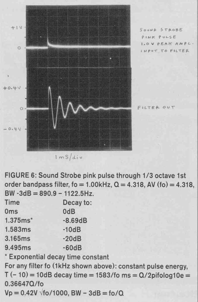
FIGURE 6: Sound Strobe pink pulse through 1/3 octave 1 st order bandpass filter,
fo = 1.00kHz, Q = 4.318, AV (fo) = 4.318.
FILTER CIRCUIT
The circuit (Fig. 8) follows the topology of Fig. 1. U1 is the input and feedback (FB) summing amp, and U2A, U2B are the integrators. VCA1 and VCA2 are the “-a” elements (controlling fo), while VCA3 is the “b” element (controlling Q Note (from Fig. 1) that Q= 1/b, so if the gain of b is zero, the Q is infinite; that is, you have an oscillator. This is because without b, there are two integrators cascaded in a FB loop. At DC the FB is inverting, but for any AC signal the integrators have a phase shift of —90° (-180° for the two cascaded). So at the frequency (fo) where the loop gain (determined by a and the value of C6, C12) is unity, the net positive FB produces oscillation.
This is the principle I used in “A Wide-Range Audio Sweep Oscillator”. The operational transconductance amps I used there (the RCAI Harris CA3280AE) are no longer available. Compared to those, the Analog Devices SSM2O18TPZ units I used in the present filter for voltage controlled amplifier/attenuator (VCA) devices have some disadvantages and advantages.
Disadvantages:
1. Less BW, about 250kHz instead of 3MHz for the CA3280AE (the latter at maximum gain where high BW is needed because fo is proportional to VCA gain). The SSM2018’s 250kHz rolloff produces a phase lag (about -5°) at 20kHz. This would increase the integrators’ desired -90° phase, which would make the filter oscillate at high intended Q values. C5 and C11 provide a phase lead, compensating this effect.
2. The SSM2018 has a low-Z voltage source output, while the CA3280 has (or rather, had) a high-Z current source output. With the latter, DC offsets decrease in proportion to the controlled signal current; also, the integrator op amps’ offset voltages don’t see a low Z from the VCA. But with the SSM2018’s low-Z output, plus the device’s own output offset (1mV typical, 15mV maximum), there’s a much more potential offset problem.

FIGURE 7: 1kHz square wave response of slope EQ. Average slope = +1.82dB/octave,
20Hz — 20kHz.

FIGURE 8: Multimode active filter.
Because the integrators are open-loop at DC, it’s only the filter’s over all negative FB that keeps offsets in check. But at low fo values, the VCAs (1 and 2) are at high attenuation (fo is 17.7kHz when the VCA is at unity gain). At 20Hz, the two VCAs combined have 118dB of attenuation (a voltage loss of 787,000:1). So there’s much less overall negative FB to control the integrators’ output DC offset. TP1 and TP2 are needed to trim the filter for acceptably low offset at low fo (to be described later).
Advantages:
1. The SSM201S has much lower distortion (0.01%) and higher gain-control precision, and a 140dB gain-control range.
2. It doesn’t need (as the CA3280 did) an external exponential converter; the VCA has a very linear dB versus control voltage relation (at pin 11).
Q CONTROL:
VCA3 (the “b” element in Fig. 1) introduces a second negative FB loop, this one around only the first integrator (U2A). This FB produces damping in proportion to the gain of VCA3. That’s why the Q is inversely proportional to VCA3’s gain. The gain of VCA3 varies from 2 (+6.0dB) for a Q of 0.5, to about 0.0085 (-41.4dB) for the maximum Q of 118 (at 20kHz in “Auto” Q mode).
The zeners (D1, D2) prevent high signal voltages from overdriving the VCA.
SLOPE EQ AND CLIP LIGHT:
Figure 9 shows the simple, switchable RC circuit that provides the +1.82dB octave up slope, reasonably uniform over the audio band. The clipping indicator light (LED 1) is useful when the filter Q is high. High Q is mainly intended for very low frequency (0.5-2Hz) Sound Strobe pulses, where you want to hear individual resonant-tone pulse responses of rooms or speakers.
However, the Sound Strobe pulse frequency goes up to 41.2Hz (the low open-E string on a 4-string bass). The filter, with high Q can tune individual harmonics out of Sound Strobe pulses above about 5Hz, but the filter’s gain is numerically equal to Q Therefore, the filter outputs can easily clip in such applications. LED1 allows you to decrease the Sound Strobe’s (or other source’s) signal amplitude, when necessary to avoid filter clipping.
CONTROL CIRCUIT
First, notice that this circuit (Fig. 1 0) uses voltages labeled “+5V PTAT” and -5V PTAT PTAT stands for Proportional To Absolute Temperature” (degrees Kelvin). This will be described later; for now, suffice it to say that this temperature compensates for the VCAs’ gain-control slope. For constant gain (or attenuation), the VCA control voltage applied must be PTAT
Switch S2 selects fo (when S3 is in the “Oct ±1 oct” position) in octave steps, from 40Hz to 10kHz. Control pot P1 adds a ±1 Octave sweep range, so S2 and P1 can control fo from 20Hz to 20k1-Iz.
When S3 is in the “Full A fo sweep” position, S2 has no effect, but P1 now tunes fo over the full 20Hz — 20kHz range.

TABLE 1: BP output pulse characteristics, “Auto” Q mode. Source is Sound Strobe
25ms exponential pulse, 1Hz rate, 2.0Vpp amplitude. T-20 is 20dB decay time,
N-20 is number of waveform cycles to 20dB decay.

FIGURE 9: EQ and clip light.
PTAT CIRCUIT
The VCAs have a control port sensitivity specification of -30mV/dB at +25° C; I measured -31.7mV/dB. But this is proportional to absolute temperature (PTAT). Therefore, to obtain tempera ture independence of the VCAs’ gains (and thus the filter’s fo and Q, the control voltages must be PTAT.
You could accomplish this by using a +3500 ppm/° C resistor (close enough to the ideal 3354 ppm/°C tempco), such as the model PT146 1k unit from Precision Resistor Co. of Largo, Fla. that I used in my 6-channel volume/balance control, which uses the same VCAs. But these cost $5 each, the filter would need two (fo and Q.), and I know of only this one source.
But there’s another way: Make the fo and Q control and bias DC voltages PTAT With the use of external fo and / or Q control signals, the above TC resistor would be needed. Here, though, the internal control pots and switches can all be supplied from PTAT DC references.
An excellent source for this is the plain old ubiquitous 1N4148 diode. If biased from a constant-current source, and the diode drop is subtracted from an appropriate constant voltage, the resulting voltage can be very close to PTAT, at least over a 0° to +50° C range (+32° to +122° F). The subtraction makes the tempco positive.
I measured the 0° to +50° C tempco of the voltage across three 1N4148 samples, at 1mA. The tempcos were within 1.1% of-2.1433mV/° C. The diode drop average was 611.38mV; highest and lowest were 616.8mV and 605.8mV.
To obtain a PTAT voltage, the output should be the product of the tempco magnitude and 298.15° K (equal to +25° C), which is 639.02mV. Then the DC reference should be the sum of this plus the typical 1N4148 drop of 611.38mV (at 1mA); this is 1.2504V ideally (the exact value isn’t that critical).
By a strange coincidence (term in vented by my father, Robert Cohn), the internal reference voltage in an LM317 regulator is very close to 1.25V. (Does National Semi know something I don’t? Of course they do, they’re experts.)
The circuit of Fig. 11 takes advantage of this. The output of the LM317 is always 1.25V (typical VREF) above the ADJ terminal, So the diode, biased negatively regarding ground, has its voltage drop subtracted from the 1.25V VREF; and without the usual external feedback needed, the LM317 output provides a very stable voltage of about +639mV at +25° C that’s proportional to absolute (°K) temperature. The 1001 load resistor ensures that the LM317’s minimum load current (3.5mA typical, 5mA maximum) is drawn.
POWER SUPPLY
The circuit in Fig. 11 is similar to that in the Sound Strobe. The rechargeable 9V batteries can be either NiCd (such as Mouser 639-N6PT) with 11OmAH capacity, or the newer NiMH types (such as Mouser 573-GP17R8H) with 17OmAH capacity. The latter type is recommended, both for its higher capacity (which will power the filter for about 2.4 hours) and its higher minimum voltage (8.4V as opposed to 7.2V for the NiCd and some other “9V” NiMH batteries).
If you prefer, you can power the filter from any ground-referenced supply of ±9V to ±15V.
TRIMMING
A. Power Supply Test:
1. With the 24V wall supply connected and S5 set to “AC,” LED2 (“AC”) and LED3 (“PWR OK”) should light. Measure the V and V voltages regarding ground; they should be in the range of ±9V to ±11V.
2. Measure the +5V PTAT voltages. They should be in the range of ±4.3V to ±5.7V, depending on the forward drop of D13 and ambient temperature.
B. Offset Trimming:
1. Set TP1, 2, 3, 4 to their approximate midpoints.
2. Set S2 to the 630Hz position (the switch’s midpoint), P1 to its approximate midpoint, and S3 to the “OCT ± OCT” position. Set P2 (the manual Q pot) fully CW (clockwise), and S4 to “manual Q”
3. Measure the DC voltages at the BP and LP outputs (re ground). If two meters are available, connect one to each output. (Accuracy isn’t needed; the cheapest meters that can resolve down to 50mV DC will do.)
4. Lower the “fo octave” setting (S2) one step at a time. At some point the offsets will increase significantly. If using only one meter, alternately observe the BP and LP offsets.
5. Lower the “fo octave” setting as many steps as possible without either offset exceeding ±2V.
6. Adjust TP1 to lower the LP offset as much as possible (it might drift around, but you should be able to null it within ±50mV).
7. Adjust TP2 to null the BP offset.
Note: It might seem strange that each trimpot affects not the op amp integrator that it feeds, but rather the opposite one. This is because the integrators’ off sets are stabilized not by local op amp FB (there isn’t any at DC), but by the overall loop. Each integrator receives DC feedback from the other one’s offset.
8. Lower the fo setting further, and repeat steps 6 and 7.
9. Continue this until the fo setting is 20Hz (S2 fully CCW (counter clockwise) and P1 fully CCW). Then null the offsets as much as possible.
C. Frequency Trimming:
Note: This requires a 20Hz — 20kHz sine wave generator and an oscilloscope (preferably) or an AC voltmeter capable of responding to the 20Hz - 20kHz range (voltage accuracy and true RIVIS response are not necessary).
===

TABLE 2: Filter data (with slope EQ switched to Flat” position).
Gain and Frequency Response - LP out: DC coupled, gain 0dB fort <<fo, gain = U at to, rolloff -12dB/octave for f >>fo.
BP out: gain = U at to, rolloffs = ±6dB/octave for liar from f. HP out: gain = (1 at to, rolloff = *12dB/octave for f<<to, HF response -3dB at 3MHz.
Maximum output ±6 peak, 4.8V RMS
Zin = 47k5, Zout = 200
THD 001%
Freq. range = 20Hz — 20kHz
Orange 0.5—30 (manual), 7.3— 118 (Auto)
Noise Out RMS
Freq. = 1kHz, U = 1: 99 (20Hz - 20kHz), 62 (A weighted)
Freq. = 20Hz, U = 1: 875 (20Hz- 20kHz), 78 (A weighted)
Freq. = 1kHz, 0 30: 250 (20Hz - 20kHz), 230 (“A’ weighted)
Output DC offset: Trimmable to ±100mV
Power Supply:
24V DC, approximately 70mA, ground isolated. May also use ground-reference supply of ±9V to ±15V, approximately ±70mA.
===

FIGURE 11: Power supply.
1. Connect the audio generator to the filter input. If a dual-channel scope is available, connect the generator also to channel 1. Trigger the scope either from channel 1 internally, or (preferable) externally from the generator’s trigger output, if it has one. Connect the scope’s channel 2 to the filter’s BP output. Set the generator’s output amplitude to about 0.5V RMS (±0.7Vpp on the scope), and frequency to 630Hz.
2. Not required, but desirable, is to monitor the source frequency with a counter, unless the generator’s frequency calibration is accurate to about ±2%.
3. Switch the slope EQ to “Flat,” S2 to its midpoint (630Hz), S3 to “Oct ± 1 oct,” and S4 to “manual Q” Set P1 to its midpoint, and P2 (manual Q also to its midpoint (Q about 5).
4. Adjust TP3 (fo trim) for a maximum output from the BP out, on channel 2 of the scope (or AC meter if a scope isn’t available). The maximum BP output voltage should be about 5x the input voltage. Note: the most accurate and sensitive way of tuning is for zero phase shift between the input and output waveforms. And the best way to see this is to switch the scope mode to “X-Y” if avail able; then at zero relative phase the ellipse will collapse to a straight tilted line.
5. Change the generator frequency to 20Hz, and set the filter fo controls to 20Hz by rotating both S2 and P1 fully CCW
6. Adjust TP4 (fo scale trim) for maximum filter output and, if possible, zero input/output phase (as in step 4).
7. Set the generator frequency to 20kHz, and the fo controls also to 20kHz (S2 and P1 fully CCW).
8. Adjust TP4 for tuning as in steps 4 and 6.
9. For the most accurate full-band tuning, alternately repeat steps 6 and 7, while periodically adjusting TP3 if necessary to offset both the 20Hz and the 20kHz settings. This can be somewhat laborious, but is needed only if the highest accuracy is desired. For most applications, the results of step 8 are acceptable.
HIGHEST Q STABILITY
The loop phase-compensating caps C5 and C11 have a strong effect on stability at 20kHz and maximum Q (which occurs in the “Auto” Q mode). To test this stability:
1. Connect a 50Hz (approximately) 1Vpp square wave to the filter, and monitor the LP output on a scope.
2. Set fo to 2.5kHz. Set the Q mode to “manual,” and set P2 (manual Q fully CCW (Q= 0.5). The output should be a LP filtered square wave, with no overshoot.
3. Turn up the Q control slowly to fully CCW. As you do, decaying ringing cycles should appear.
4. Switch S4 to “Auto” Q mode. At fo settings above 1kHz (such as the 2.5kHz it’s set to now), the Q should increase when switching S4 from “manual” to “Auto.” This should make the ringing’s decay longer.
5. Set P1 to about two-thirds of the way up, and switch S3 to “Full P1 Sweep.”
6. Slowly turn up P1. When it’s up fully CW, the filter might break into continuous oscillation at 20kHz. If this happens, C5 needs to be increased. Increasing it from 100pF to 120pF should be enough. Increasing it too much will reduce the maximum avail able Q.
7. The ideal is to have a value of C5 (C11 has the same effect) that produces a long ringing decay at 20kHz fo, without oscillating. CS can be a trimmer cap with a minimum value of 80pF or less, and a maximum value of at least 150pF.
= = =
SPEAKER CROSSOVER COMPARISON EXAMPLE
I found the filtered Sound Strobe pulses to be very revealing of a speaker CO alignment. I could easily hear the frequency delay dispersion of a woofer/mid CO that had very flat amplitude/frequency response, the Swans Mi/Scan-Speak sub unit.
The raw Sound Strobe pulses, particularly the LF, 2Sms exponential, and 830 exponential pulses, clearly revealed the 220Hz CO’s transient delay dispersion. But filtering the 2Sms exponential pulse with the BP filter fo at 220Hz made the delay dispersion more audible. I compared the Swans system to a full-range Seas coincident driver in a sealed box. With a filter Q of 30, the Swans made an audible separation between the transient attack and the resonant tone. But with the Seas, the sound was coherent; I could picture an actual drum skin sound.
Interestingly, there were many positions in the room where I could hear a standing wave null, almost removing the pulse’s 220Hz tonality, with both speakers. However, I could still hear the superior “live drum-like” transient response of the full-range Seas, regardless of room effects.
This correlates with recorded drums and string bass sounds, but I must have to listen for the Swans/sub delay-smearing effect. With the filtered Sound Strobe pulses, it’s immediately recognizable.
Figure 13 shows an electronic representation of this effect: The “A” waveform is the 25ms exponential pulse, filtered with fo = 232Hz and Q= 0.65; that Q produced the cleanest pulse without significant overshoot.
Waveform “B” is this pulse through a three-stage non-resonant all-pass network, with its fo (center of its phase/frequency graph on a log frequency scale) at 232Hz, the same as the BP filter’s fo. The all-pass network’s group delay ranges from 4.12ms for frequencies much lower than 232Hz, to 2.06ms at 232Hz, and approaches zero at frequencies much above 232Hz.
This all-pass response is similar to a fourth-order CO that (like the all-pass) has a flat amplitude/frequency response. Note how the clean transient “A” waveform is smeared with frequency selective delay The original waveforms peak is delayed about 3.4mS, and also reduced in amplitude. Unlike some measurements, this effect is as audible as it looks.
= = =

TABLE 3: Parts List
= = =
Table 3 is the parts list. Figure 12 shows my suggested enclosure panel component layout. Please let audioXpress know whether you would find this filter useful. If there’s enough interest, a kit and assembled product may become available. Table 4 shows bandwidth versus Q data.
CONCLUSION
The wide range of transient pulses shown in this article can be very useful test signals for directly hearing speaker time mis-adjustment, frequency response anomalies, and spatial image coherence; and also the effects of room acoustics. The principal features are:
1. The raw Sound Strobe pulses are best for hearing wideband transient response and overall freedom from (or degree of) speaker coloration, and the smoothness of room acoustics (freedom from discrete echoes).
2. The filtered pulses allow frequency tuning of all the audible effects de scribed. The Q control allows a wide range of resonant tonality (including none) to be selected.
3. The precise-transient resonant tone pulses, because of their resemblance to natural acoustic sounds, provide good correlation with musical re production quality, but with very high sensitivity and repeatability.

TABLE 4: Normalized and octave bandwidths as a function of Q.

FIGURE 12: Suggested enclosure panel component layout, based on front panel
dimensions = 9.0”x 2.1”.

FIGURE 13: Simulated woofer/mid crossover effect on filtered Sound Strobe
pulse.
= = = =