PART 1--REAL VERSUS IDEAL COMPONENTS

Major Edwin Armstrong, who was undoubtedly the most prolific and down-to-earth of the radio " pioneers, " was fond of repeating a saying which went something like this:
It ain't the things you don't know that get you into trouble; it's the things you know for sure--that ain't so.
Armstrong went on to prove the wisdom of that proverb by singlehandedly inventing FM radio, even though the theoretical experts already "knew for sure" that FM radio wouldn’t work.
Electronics technicians today often get into trouble because there are too many things that they "know for sure" about electronic components that in reality "ain’t so."
Ideally, for example, hookup wire has zero resistance, and a coil whose inductance is measured as 10 uH at 1 MHz will also be 10 uH at 10 MHz. Such idealizations are commonly applied in the practice of electronics, and indeed a good case could be made that the practice of the art as we know it would be impossible without such simplifying assumptions. Eventually, however, the technician is bound to run afoul of his assumptions and he will have to recall that his initial analysis was based on an idealized mathematical model of a certain device which cannot possibly reflect all the properties of the actual physical component.
Then he will have to ask himself: "What are the real properties of this component? How are they different from the mathematical model? Under what conditions is the model essentially valid, and when must I discard the model and look for the nonideal effects?"
He may find that the near-zero resistance of hookup wire is not near-zero enough in the case of 5-A current pulses, and that the distributed capacitance in the windings of a 10-uH coil cancels out the majority of the coil's reactance at 10 MHz, even though it was negligible at 1 MHz.
The purpose of this unit is to give the technician some awareness of the nonideal effects in common electronic components. In many cases, these concepts will not be needed, as the behavior of the real component will be close enough to the ideal to make the idealized model valid. However, when an "impossible" situation comes up in troubleshooting--say a substantial voltage drop across a supposedly zero-resistance wire, or a transistor that refuses to saturate even though the beta formula says that it has more-than-enough base dive--then it will be time to remember the difference between the ideal and the real.
PROPERTIES OF REAL WIRE AND CABLE
1.1 CONDUCTIVITY OF WIRE
The actual dc resistance of various sizes of solid copper wire is given in Fig. 1-1.
For resistance to ac, be sure to read Section 1.4 on skin effect. Stranded wire is sized to have a similar cross-sectional area, and hence equivalent dc resistance, as equivalent-sized solid wire. For example, 10 strands of No. 30 wire would have an area of 1000 circular mils, and would be called No. 20 stranded wire, since No. 20 wire has about the same area (1020 circular mils, to be exact).
Other Metals: The resistance of other metals relative to copper is given in Fig. 1-3.
Notice, for example, that a length of aluminum wire has 1.64 times the resistance of a copper wire of the same length and diameter.
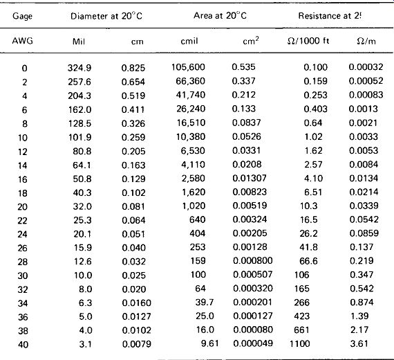
FIGURE 1-1 Resistance and standard sizes of copper wire.
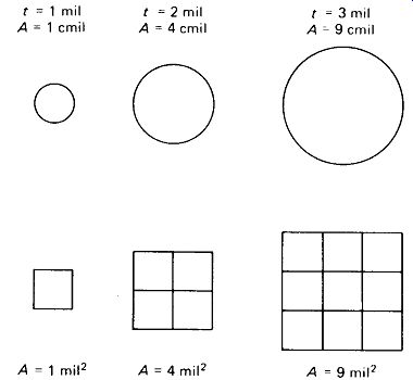
FIGURE 1-2 Area in circular mils equals the square of wire diameter in mils
(thousandths of an inch).
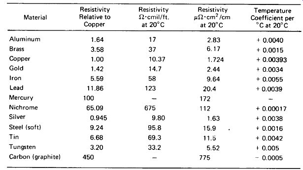
FIGURE 1-3 Relative resistance of various conductors (copper- 1.000) and
temperature coefficients of resistance.
Circular Mils: The cross-sectional areas of the wires in Fig. 1-1 are given in circular mils. One circular mil is the area of a circle 1 mil in diameter. As illustrated in Fig. 1-2, circular-mil area is then simply the square of wire diameter in mils (thousandths of an inch).

(1-1)
Calculating Wire Resistance: If necessary, the resistance of a length of wire can be found directly from the following formula:
(1-2)
where R is the wire resistance in ohms, p the resistivity of the wire material in ohms-cmil/ft (Fig. 1-3), / the length of the wire in feet, and A the cross-sectional area in circular mils (square of diameter in mils, or from Fig. 1-1).
EXAMPLE 1-1 What is the dc resistance of 5280 ft of No. 26 stranded copper wire at 25°C?
Solution From Fig. 1-1, each foot has 0.0418 ohm:
R = 5280 ft x 0.0418 i/ft = 220.7 ohm
EXAMPLE 1-2
What is the resistance of 10 ft of No. 22 Nichrome wire?
Solution
From Fig. 1-1, 10 ft of No. 22 copper wire has a resistance of 0.165 0. From Fig. 1-3,
Nichrome wire has 65.09 times the resistance of copper, so R = 0.165 Q x 65.09 = 10.7
EXAMPLE 1-3
The diameter of a solid steel conductor measures 0.25 in. What is the resistance of 500 ft of this conductor?
Solution
[…]
1.2 TEMPERATURE EFFECTS AND CURRENT CAPACITY OF WIRE
Figure 1-3 shows that the resistance of metal conductors increases at higher temperatures. Copper wire, for example, undergoes an increase of 0.393% for each degree Celsius rise in temperature. For a 100°C rise (the rise from freezing to boiling of water) this would amount to a resistance increase of 39%.
Temperature-Stable Alloys: For applications where highly temperature-stable resistances are required, special alloys (usually of copper with nickel) are available which have temperature coefficients below 0.00002 per ° C.
For such metals, resistances can be held stable to better than 0.1% over the normal range of human-environment temperatures.
Semiconductor Temperature Coefficients: Nonmetals, such as carbon, generally have a negative temperature coefficient of resistance, meaning that their resistance goes down as temperature goes up.
The semiconductor materials, "doped" silicon and germanium, have temperature coefficients which are large and negative, but are otherwise difficult to predict because of their extreme dependence on very small impurity contents. The resistance versus temperature curve for a typical slab of silicon semiconductor is given in Fig. 1-4. The rapid change of resistance with temperature is exploited in the manufacture of thermistors for temperature measurement and control.
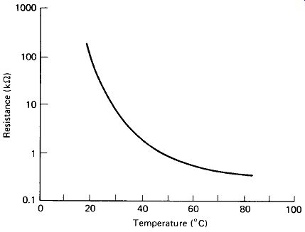
FIGURE 1-4 Resistance versus temperature for a typical silicon thermistor.
Maximum Current versus Wire Size: The recommended maximum currents for various sizes of copper wire may be obtained from Fig. 1-5. The lowest line (10° C rise) should be used for systems that must run cool. The center (35° C) should be thought of as the maximum for most common types of insulated wire, since it represents operating temperatures in the neighborhood of 150° F. The top (140°C rise) line represents final wire temperatures of about 320°F, and should be used only for bare wire suspended by high-temperature insulating supports.
The basic chart is for two or three insulated wires in a bundle, and the allowable currents should be reduced by the factors given in the table accompanying Fig. 1-5 for larger bundles.
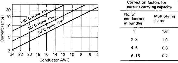
FIGURE 1-5 Maximum current versus wire size of copper wire for various maximum
temperature-rise limits. (Courtesy Potter and Brumfield Division, AMF Inc.,
Princeton, Ind.)
1.3 INSULATION AND VOLTAGE RATING OF WIRE
Any insulating material can be made to conduct if enough voltage is applied across it to rip the normally well-bound electrons loose from their atoms. If a fairly large current is allowed to flow through such an insulation breakdown, enough heat may be generated to permanently destroy the insulator. Figure 1-6 shows that not all materials are alike in their ability to resist voltage breakdown, and that just about any solid insulator is better than air. The values given do not include a safety factor, so the wise designer will assume the worst-case insulating strength to be one-fifth to one-tenth of the value given.
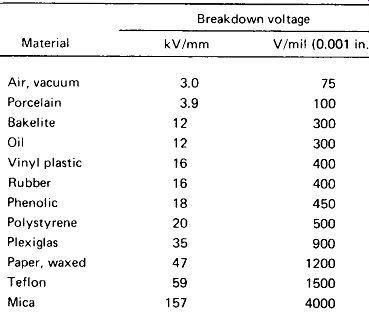
FIGURE 1-6 Breakdown voltages for various common Insulators.
In choosing an insulating material, it is well to consider the possibility of environmental deterioration as well as the original insulating ability. Rubber can become cracked and brittle with age, oil can become contaminated, polyvinyl chloride materials can embrittle under exposure to sunlight, and air can be laden with salt spray and humidity.
Arcing from a Sharp Point: Electric charge accumulates at a sharp point, but spreads evenly over a smooth surface. The results of this are depicted in Fig. 1-7.
Four different conductors were held 2 mm from a metal plate, and the voltage required to arc the air between them was measured. When the conductor was a smooth sphere, a voltage of 8 kV was required. When a 90° bend in a No. 24 wire was used, 5 kV caused an arc. But when a sharply pointed No. 24 wire was used, arcing started at only 2.5 kV. A piece of insulating sleeving on the wire stopped all arcing. Therefore, when constructing high-voltage systems, the technician should:
1. Cut or file off all sharp metal and wire points.
2. Leave smooth, rounded solder joints with no sharp protruding solder "tails."
3. Use insulating sleeving on any bare high-voltage conductors.
4. Cover, coat, or paint surfaces where arcing is likely to be a problem.
Special "corona dope" compounds are available for this purpose.
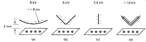
FIGURE 1-7 Test results: arcing is less likely to occur from a smooth or
insulated surface than from a sharp point.
1.4 SKIN EFFECT AND STRAY INDUCTANCE OF WIRE
At high frequencies, the magnetic fields within a wire become such as to force all charge carriers to flow at the surface of the wire, leaving the center of the wire useless as a conductor. This phenomenon, known as the skin effect, means that the resistance of a wire conductor increases at high frequencies.
At dc and low ac frequencies the conductivity of a wire is proportional to its circular-mil area (diameter squared), and heavier wire really does have much better conductivity. However, at radio frequencies conductivity is proportional to surface area (which is directly proportional to diameter), and the advantage of heavier wire is less pronounced. Larger-sized wire begins to suffer from the skin effect at a lower frequency because its central core is farther removed from the skin.
Calculating Skin Effect: Although the current density under the skin effect actually drops off exponentially from the surface toward the center of the wire, the effect is the same as if a uniform current density were confined to a conductive surface with a thickness 5, called the skin depth. This is illustrated in Fig. 1-8(a).
Actually, the current density is 38% of its full value at the skin depth. For round copper conductors, skin depth can be calculated by V? where S is in centimeters and / is in hertz. For other metals, the depth can be determined by multiplying by the square root of the relative resistivity from the table of Fig. 1-3. Aluminum, for example, has a skin depth of Vl.64 = 1.28 times that of copper. Skin depth is important because it determines the heaviest solid wire that can be effectively employed at a given frequency. If the wire has a diameter greater than 25, the center of the wire is relatively useless.
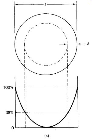
FIGURE 1-8 Wire impedance increases at high frequencies: (a) skin depth
6 and current distribution in a round wire at high frequency.
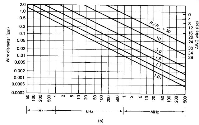
FIGURE 1-8 (b) Skin effect for straight conductors versus wire size and
frequency.
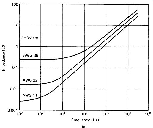
FIGURE 1-8 (c) Measured values of Impedance versus frequency for 30-cm lengths
of various wire sizes.
EXAMPLE 1-4 What is the maximum effective diameter of a copper wire for 60-Hz power transmission?
Solution
(1-3)
The actual resistance of a copper wire under skin effect can be determined from Vf…
(1-4)
where R is in ohms, / is in hertz, and t and / are thickness and length, respectively, in any commensurate units (both inches, both centimeters, or whatever). For other conductors, multiply by the square root of the relative-resistance value in Fig. 1-3.
Silver, for example, has a skin-effect resistance of V0.945 or 0.972 times that of copper. Figure l-8(b) shows the ratio of skin-effect resistance to dc resistance as a function of wire size and frequency, and may be used in place of Equation 1-4 for obtaining rough estimates.
EXAMPLE 1-5 What is the voltage loss across a 200-ft length of RG-58 coax feeding a 50-0 load at 30 MHz?
Solution
Assuming the loss to be primarily in the 0.033-in. diameter center conductor, we find its skin-effect resistance.
This situation was set up in the laboratory where a V„/Vin ratio of 0.58 was measured at 30 MHz.
Proximity Effect: The skin-effect formulas are accurate only for round conductors running in a straight line. When the wire is wound into coils, additional magnetic fields cause further increases in wire resistance. This proximity effect is difficult to predict, but it is by no means negligible. The following factors will serve as a rough guide to the proximity effect to be expected.
pretty (actual) Coil Configuration /{ (calculated) Single-layer, spaced 5 to 20 1.5 to 3 diameters between windings
Single-layer, close-wound 5 to 15 Multi-layer winding 15 to 100
A summary of the most common situations may be helpful. At 60 Hz, skin effect does not become evident even in transformer coils except in wire sizes larger than about AWG 4. In audio transformers up to 10 kHz, skin effect is negligible for wire sizes smaller than about AWG 24. Such large wire sizes are quite uncommon, making dc resistance satisfactory for most power and audio trans former calculations. For most common wire sizes skin effect or proximity effect is evident by 100 kHz, and there are few practical situations above 1 MHz where skin-effect resistance is not many times dc resistance.
Combating Skin Effect: Stranded wire suffers from skin effect to about the same degree as does equivalent-sized solid wire. (The advantage of stranding is the ability of the wire to flex without breaking.) However, if each strand is separately insulated from the others, with the strands tied together at each end, some relief from skin effect is obtained. Such wire is called litz wire and is effective for winding high-Q coils in the 0.1- to 2-MHz range. Below 0.1 MHz, stray capacitance between the strands washes out the benefits of litz wire.
Where energy loss is critical and strength is important, copper-clad steel wire is often employed. The copper coating, one or two skin depths thick, provides conductivity while the steel provides strength. For large-diameter conductors, hollow tubing is lighter, cheaper, and just as conductive, provided that its thickness is two skin depths or more. Flat copper strap also provides greater surface area with less volume of metal. At high radio frequencies a very thin silver plating on a metal or plastic support provides as much conductivity as possible, if the plating is several times the skin depth.
Stray Inductance of Wire: In practice, skin effect in hookup wire is usually masked by the stray inductance of the wire, which may be anticipated to be about 0.04 uH/cm or 1 uH/25 cm.
Skin-effect resistance in hookup wire is typically an order of magnitude (factor of 10) less than the reactance caused by stray inductance. Figure 1-8(c) shows measured values of total impedance for three sizes of solid copper wire from low audio to high radio frequencies. Notice that a simple 1-meter test lead of No. 22 wire has an impedance in the vicinity of 60 ohm at 10 MHz.
Any two conductors separated by an insulator form a capacitor, and adjacent lengths of hookup wire fill this requirement in every respect. The following list will be helpful in estimating the stray capacitance between various types of conductors.
-------------------
Two No. 22 solid PVC-insulated wires 40 pF/m adjacent in a bundle
Two No. 22 wires twisted 1 turn/cm 46 pF/m
One No. 22 wire held flat against a 65 pF/m metal chassis
Two No. 22 wires held 2 cm apart 12 pF/m
Two conductors of No. 18 lamp cord 50 pF/m
Shielded wire; No. 22 stranded center 300 pF/m conductor to braid RG-58/U coax cable (7 mm diameter) 88 pF/m 300 U TV twin lead 20 pF/m
Tubular capacitor, 2 cm diameter, 5 cm long; 10-20 pF outside foil to metal chassis
--------------------
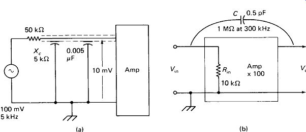
FIGURE 1-9 Common problems from stray capacitance; (a) shielded microphone
cable attenuates audio highs; (b) small stray feedback capacitance causes
self-oscillation in an amplifier.
High-Frequency Loss on a Microphone Line: Cable capacitances may prove far from negligible in many practical cases. For example, at 5 kHz, 20 m of heavy shielded wire may present a reactance to ground of 5 k ohm. The popular low-cost crystal microphones typically have an internal impedance of 50 k ohm. Figure 1-9(a) illustrates how the loading effect of the cable capacitance may cause the higher audio frequencies to be attenuated (by a factor of about 10 in this case) before they reach the amplifier input. Of course, the problem can be readily solved in a number of ways-use a low-impedance microphone; use a step-down transformer at the "mic" and a step-up transformer at the amp; put an emitter follower or FET amplifier stage in the mic case; use special hi-Z shielded cable; and so on. But the first step in solving any problem must be to identify its cause.
Self-oscillation in an Amplifier: Figure 1-9(b) illustrates another common problem caused by stray capacitance. The input and output leads of the high-frequency amplifier depicted pass within a few centimeters of each other for a short distance, resulting in a feedback capacitance of 0.5 pF. At about 300 kHz this capacitance has a reactance of 1 M-ohm and the voltage division of Xc with provides a feedback voltage equal to the input voltage. If the phase shift within the amplifier is right, the result will be self-oscillation. To avoid this problem, the input and output wires of any amplifier should be kept completely away from each other and the components on the circuit board should be laid out to implement this. Vertical shield plates can be mounted across a transistor and soldered directly to the chassis to screen the input from the output. Keeping the amplifier input impedance low reduces the feedback ratio and thus helps prevent oscillation.
Coupling between Shielded Cables: Shielded wire and coaxial cable can greatly reduce unwanted coupling between wire runs, but you should guard against the feeling that nothing can get into or out of a shielded cable. Figure 1-10 shows the results ol some laboratory tests using RG-59/U coax cables. In Fig. 1-10(a) an unshielded length of hookup wire run along the outside of the coax cable picks up as much as 25% of the cable' s signal at certain frequencies. In Fig. 1-10(b), two lengths of coax couple as much as 3% of the signal from one to the other at high frequencies when held close together.
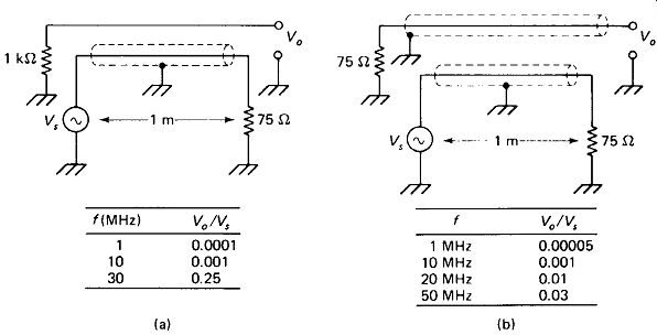
FIGURE 1-10 Lab test: (a) up to 25% of the voltage on a coax cable la coupled
to an adjacent high-impedance wire; (b) up to 3% is coupled between two coax
lines 1 m long.