Vertical pulse height represents signal strength and horizontal pulse position represents frequency. Learn more about this important but frequently overlooked instrument.
By FERNANDO GARCIA VIESCA
THE SPECTRUM ANALYZER LETS YOU view the frequency domain the same way the oscilloscope lets you view the time domain. This article is a primer (or refresher) on the spectrum analyzer, an extremely powerful and versatile test instrument that is frequently overlooked by many who have never taken the time to explore its special properties.
Long considered too specialized and too expensive for general use, the spectrum analyzer has recently become an important test instrument in cable television, computer networks, digital radio, and automated component testing. However, for years it had been a well established instrument in radio and radar transmitter design and maintenance.
Government requirements mandating the control of electromagnetic interference (EMI) have made the spectrum analyzer a factory-production and quality control tool in the manufacture of many different kinds of electrical and electronic equipment.
The selection of the appropriate spectrum analyzer for a given task will depend on such factors as the frequency sweep rate, frequency sweep range, bandwidth, and the center frequency of its intermediate frequency system. Other considerations are the bandwidth of its video amplifier and the analyzer's overall sensitivity.
Spectrum analyzers are useful in the analysis of continuous-wave (CW) signals, amplitude-modulated (AM) signals, frequency-modulated (FM) signals and pulse-modulated signals: pulse-amplitude modulated (PAM), pulse-width modulated (PWM), and pulse position modulated (PPM) signals.
Before discussing the spectrum analyzer and how it works, a review of some of its basics will be useful. Figure 1 illustrates two different ways of looking at the same signal. The waveform viewed at the left is an instantaneous voltage plotted against time, as seen on an oscilloscope. The view at right shows the same waveform, but here the voltage is positioned with respect to frequency rather than time.
A complex signal has more than one frequency component (spectral line), which indicates the amount of energy that is present at each frequency. The more complex the waveform, the greater the number of spectral lines.
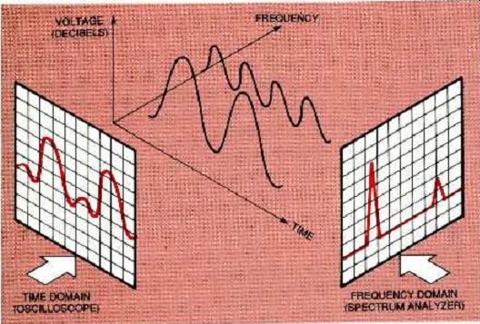
FIG. 1--TIME-DOMAIN MEASUREMENTS made with an oscilloscope (left) are
compared with frequency domain measurements that can be made with a spectrum
analyzer (right).
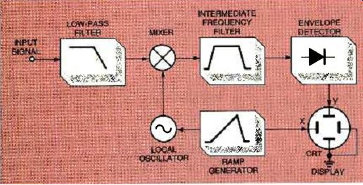
FIG. 2--SIMPLIFIED SPECTRUM ANALYZER BLOCK DIAGRAM. The input signal
Is mixed with local oscillator (LO) signal in the mixer. The intermediate
frequency (LO) is filtered, detected and displayed on the CRT's vertical
axis. The ramp generator triggers the CRT's time base and the LO.
According to the French mathematician and physicist Jean Fourier, any time domain electrical signal consists of one or more sine waves, each with its own frequency, amplitude, and phase. As a result of his insight, it was found that any complex time-domain waveform can be broken down into separate sine waves that can be evaluated separately. In effect, any time domain signal can be transformed into its frequency-domain equivalent.
Theoretically, any signal must be evaluated for an infinite length of time when making a transformation from the time to the frequency domain. However, in practice, it is assumed that the behavior of a signal for time intervals ranging from milliseconds to a minute will give a reasonably accurate indication of the waveform's long-term characteristics.
Time vs. frequency domain
Time-domain measurements from an oscilloscope provide an overall view of the signal waveform, including such characteristics such as pulse rise and fall times, overshoot, and ringing. By contrast, the spectrum analyzer provides a panoramic display of the signal distribution in a selected portion of the radio frequency or microwave bands. The display can show the presence or absence of signals of interest, their frequencies or harmonic content, frequency differences, relative amplitudes, and the modulation form, if any.
In the United States and most of the advanced countries of the world, radio equipment must meet government-imposed standards for spectral purity.
The spectrum analyzer permits the viewing of the bandwidth of the modulated signal, and it also gives an immediate indication of the harmonic content of a transmitter's signal.
Harmonics of the carrier signal might interfere with other systems operating at the same frequencies as the harmonics.
Improper RF transmission conditions such as splatter or over modulation can be easily seen as excessive bandwidth. These deviations can be observed on a spectrum analyzer. This is helpful in making adjustments and corrections.
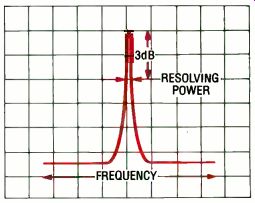
FIG 3--TYPICAL CONTINUOUS-wave signal
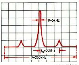
FIG. 4--SINGLE-TONE AMPLITUDE modulated signal.
How does it work?
There are four basic spectrum analyzer architectures: bank of filters, fast Fourier transform (FFT), wavemeter, and swept spectrum or superheterodyne.
Each has its own set of strengths and weaknesses, but in this article only the superheterodyne architecture will be discussed.
Figure 2 is a simple block diagram of a superheterodyne spectrum analyzer. It is essentially a narrow-band superheterodyne receiver that is repeatedly swept in frequency over a selected portion of the RF band. Heterodyne means to mix signals together to produce sum and difference frequencies. Superheterodyne has the same meaning except that the signals being mixed are above the audio range.
The ramp (or sweep) generator generates a sawtooth (or ramp) waveform that tunes the local oscillator (LO). A form of frequency generator, it is swept linearly between two frequency limits. At the same time, the ramp generator also deflects the CRT beam horizontally across the screen from left to right. The local oscillator output is fed into the mixer.
The input signal is passed through a low-pass filter to the mixer, where it is mixed with the LO output. The output of the mixer includes not only the input and LO frequencies, but also their harmonics and sums and differences.
Only those mixed signals that fall within the passband of the intermediate frequency (IF) filter will be passed on to the envelope detector, represented here as a diode. The output of the envelope detector is amplified and applied to the vertical plates of the cathode-ray tube (CRT) to produce a vertical deflection on the CRT screen.
The CRT screen typically has a graticule or overlay grid of lines-ten horizontal and eight or ten major vertical divisions spaced one centimeter apart.
The horizontal axis is calibrated in frequency that increases from left to right.
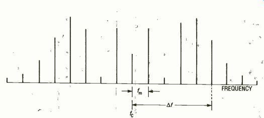
FIG. 5--SINGLE-TONE FREQUENCY-modulated tone where fm equals the modulating
frequency.
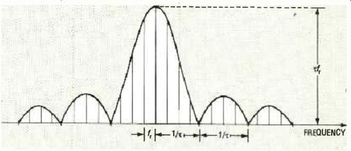
FIG. 6--PULSE-MODULATED SIGNAL where fr equals the pulse repetition
frequency and 7 equals the pulse width.
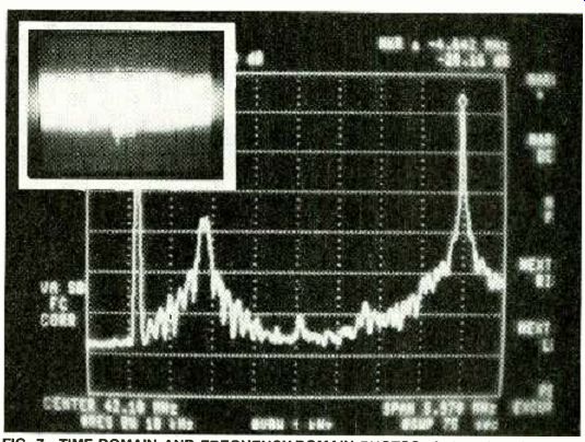
FIG. 7--TIME-DOMAIN AND FREQUENCY-DOMAIN PHOTOS: A time-domain waveform
as displayed on an oscilloscope (inset), and frequency-domain waveform
of the same signal as displayed on a spectrum analyzer.
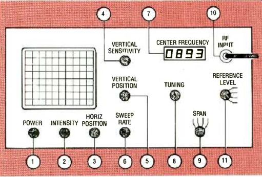
FIG. 8--SPECTRUM ANALYZER FRONT PANEL: The controls of a basic model.
1. POWER switch turns power on and off.
2. INTENSITY controls brightness of the display.
3. HORIZONTAL POSITION shifts the display on the screen.
4. VERTICAL SENSITIVITY selects an amplitude sensitivity.
5. VERTICAL POSITION moves the CRT display vertically.
6. SWEEP RATE controls the sweep speed across the CRT
7. CENTER FREQUENCY is a readout of center frequency.
8. TUNING centers the frequency on the CRT display.
9. SPAN controls the spectrum display width.
10. RF INPUT accepts the signal to be observed.
11. REFERENCE LEVEL sets waveform to the graticule top.
More advanced models have additional function knobs, switches, and pushbuttons.
PORTABLE SPECTRUM ANALYZER from Hewlett-Packard covers the RF and microwave frequency range from 9 kHz to 22 GHz. It offers frequency-synthesized accuracy of 7.6 kHz at 1GHz. Second- and third-order dynamic ranges are 77 dB and 90 dB, respectively. Memory cards can quickly transform the unit into an application-specific instrument.
Signal treatment
If a spectrum analyzer receives a continuous-wave signal, the trace is a plot of the bandpass characteristic of the intermediate-frequency amplifier, as shown in Fig. 3. A single response will show up on the screen, and the resolving power of the analyzer is equal to the 3 dB bandwidth of the intermediate-frequency amplifier.
The spectrum of a single-tone, amplitude-modulated signal will consist of the vertical response representing the original carrier frequency plus a pair of side frequencies, one above and the other below the carrier, as shown in Fig. 4. The amplitude of either sideband voltage with respect to the carrier voltage is m/2, where m is the percentage modulation. The frequency difference between the carrier and either sideband is equal to the modulating frequency, as shown in Fig. 4.
If the modulating wave is complex, each frequency component in the wave contributes a pair of side frequencies to the spectrum. These side frequencies are located at equal distances on each side of the carrier, and they are spaced away from the carrier by the modulating frequency of the wave under study.
In frequency modulation, a single modulating tone will produce a carrier with an infinite number of side bands. Nevertheless, the spectrum will be symmetrical about the center frequency, as shown in Fig. 5.
Pulse modulation is a special case of amplitude modulation in which the carrier is on during selected intervals (pulses), and is off between these pulses.
It is done to increase the ratio of peak to average power in the modulated wave as in pulsed radar or to encode a signal as in pulse code modulation (PCM). Without going into the mathematical derivations, it is sufficient here to point out that the spectral display of a pulse-modulated carrier is that of a large magnitude lobe centered on the carrier's center frequency with side lobes of diminishing amplitude spaced equidistantly on either side of the center frequency, as shown in Fig. 6.
Graphic records
Figure 7 show a photograph of a 45.75 MHz, video-modulated, intermediate-frequency signal from a tuner, taken from an oscilloscope display. It can be seen that the modulation makes it impossible to freeze the display on this time-domain oscilloscope picture. Peak–to-peak voltage is the only measurement that can be accurately made.
Figure 7 also shows a spectrum analyzer presentation of the same waveform. It is now possible to recognize (reading from left to right) the audio sub-carrier, the modulated 3.58 MHz chroma subcarrier, and the modulated video carrier with its sidebands. Because this is an IF output, the audio subcarrier is lower in frequency than the video signal.
From that waveform it is possible to measure the video carrier level, the audio carrier level below video, the frequency of the video carrier, and the frequency span from the video to the audio carriers. This is particularly important because an off-frequency audio subcarrier causes an annoying distortion on the TV screen called "beats." With tedious adjustments and care, it might be possible to measure modulation depth, audio deviation, and signal-to-noise ratio. However, none of these can be measured with a conventional oscilloscope.
Basic control functions
Figure 8 shows the front face of a spectrum analyzer with a minimum number of controls.
The input connector is usually placed on the front panel. The power switch typically has a lamp nearby to indicate if the power is on or off.
The controls includes knobs for setting waveform intensity, horizontal position, vertical sensitivity, vertical position, and sweep rate. A tuning knob sets the center frequency, which is displayed on a liquid crystal display panel. SCAN WIDTHS or SPAN (MHz /div) sets the scan width and REFERENCE LEVEL (dBm) sets reference level. Some instruments have a knob for setting for BANDWIDTH (BW normal or wide). The vertical axis is calibrated in amplitude. Most analyzers offer a choice of linear scale calibrated in volts or power, or a logarithmic scale calibrated in decibels. The log scale offers a much wider usable range. The top line of the graticule is normally assigned as the reference level, and scaling per division permits the assignment of values to other graticule locations.
This permits the measurement of both the absolute signal value or the amplitude difference between any two signals.
The cost of spectrum analyzers has been declining over the past decade while their performance, efficiency and reliability has been improved. The availability of higher levels of integrated circuitry has permitted lower power consumption.
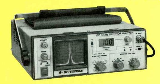
The battery-portable 2610 spectrum analyzer from B + K Precision, shown on the first page of this article, covers the frequency range of 1 MHz to 1 GHz. It offers a fixed 1 MHz bandwidth, regardless of scan width. This, B+K says, simplifies the observation of video, television, and cable television signals. This B +K instrument is considered to be a general purpose analyzer.
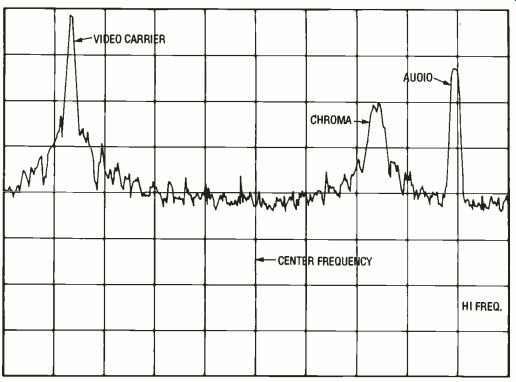
FIG. 9--THE STANDARD V DEO CARRIER WAVEFORM (V) shown with its chroma
(C), and audio (A) subcarriers at higher frequencies. Table 1 gives the
basic settings.
---------------TABLE 1
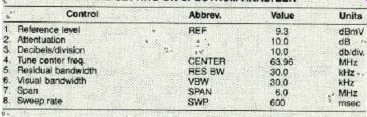
INITIAL SETTING ON SPECTRUM ANALYZER
Control Abbrev. Value Units
1. Reference level REF 9.3 dBmV
2. Attenuation 10.0 dB
3. Decibels /division 10.0 db /div.
4. Tune center freq. CENTER 63.96 MHz
5. Residual bandwidth RES BW 30.0 kHz
6. Visual bandwidth VBW 30.0 kHz
7. Span--SPAN 6.0 MHz
8. Sweep rate SWP 600 msec
-------------

FIG. 10--RETUNING THE CENTER FREQUENCY from 63.96 to 66 33 MHz shifts
the trace toward the higher frequency. All other settings remain the
same.
--------------
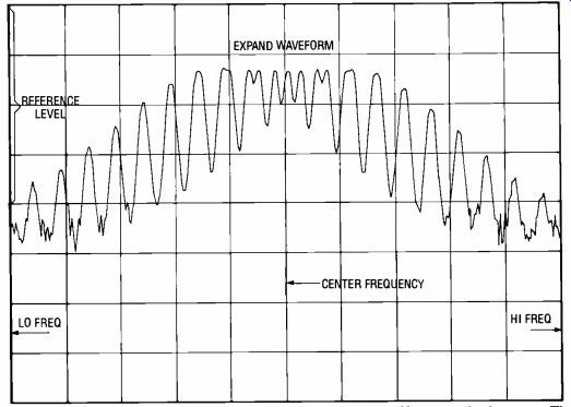
FiG. 11--DECREASING THE SPAN FROM 6.0 MHz to 200.0 kHz expands the trace.
The center frequency has shifted from 66.33 to 66.31 MHz, and the sweep
has decreased from 600 to 20 milliseconds. All other settings remain
the same.
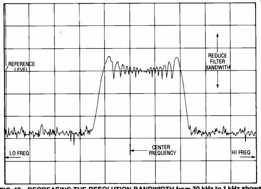
FiG. 12--DECREASING THE RESOLUTION BANDWIDTH from 30 kHz to 1 kHz shows
the true amplitude of the sidebands. The sweep has increased from 20
milliseconds to 18 seconds. All other settings remain the same.
The high end of the market is represented by the 8593E from Hewlett-Packard. It is a spectrum analyzer that can make frequency measurements at 22 GHz. One of a family of HP spectrum analyzers, it is designed so that relatively unskilled operators can make routine specialized precision measurements on the factory floor just by pushing a few front-panel buttons.
Some of the high-end models include microprocessors which permit the display of alpha-numeric legends on the CRT screen to verify settings. It also permits the selection of amplitude units on either log or linear scale.
Some models have movable cursors that can be located at any point on the displayed trace so that the frequency or amplitude values at that point will be displayed. Digital storage of the displayed waveform eliminates display flicker at the sweep rate.
Pushbuttons have replaced control knobs on some models, and battery-portable analyzers are also becoming popular.
Advanced spectrum analyzers have provision for "personality cards," which, when inserted, dedicate the instrument to specific applications and minimize the number of settings and adjustments that must be made. This feature permits relatively unskilled operators to carry out precise production-line or laboratory measurements.
Control settings
The two basic settings that must be made when operating an oscilloscope are vertical volts per division and horizontal time (seconds) per division. Of course, other setting such as trigger level, horizontal and vertical position, and certain other enhancements will give the clearest possible waveform.
By contrast, when operating a spectrum analyzer, there are more required settings. These include the vertical reference level, horizontal center frequency, horizontal sweep time, and resolution bandwidth.
Some analyzers offer a choice of vertical reference level units.
These include decibels referred to a milliwatt (dBm), to a nanovolt (dB nV), to a microvolt (dB RV), and to volts and watts.
A choice can also be made between a 50-ohm and a 75-ohm input impedance.
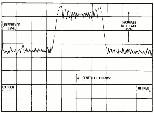
FIG. 13--DECREASING THE REFERENCE LEVEL from 9.3 dBmV to-12 dBmV elevates
the waveform. All other settings remain the same.
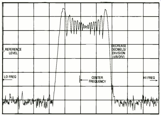
FIG. 14--DECREASING THE DECIBELS /DIVISION value from 10 to 5 dB /div
amplifies the waveform. All other settings remain the same.
Figure 9 is a rendering of an actual spectrum analyzer waveform of a radio-frequency video carrier reproduced with an X-Y plotter. Notice that because it is a radiofrequency signal and not an intermediate-frequency video signal, the carriers are in their normal positions-the audio has a higher frequency than the video signal. Table 1 gives the initial settings.
Referring back to the spectrum analyzer front-panel diagram, Fig. 8, the following information can be gained: Reference level-The reference level is given at the top of the graticule. All other voltage or power levels are below that maximum level. The REFERENCE LEVEL knob adjusts the input attenuator and IF gain so that the top graticule corresponds to the indicated signal level. Calibrations might be in dBm or dBmV. Vertical sensitivity or scale-selects the amplitude sensitivity of the graticule. Typical selections are 10 dB /div or 2 dB/ div.
Tuning-sets the mean or center frequency of the display.
Some models display this value separately on a liquid-crystal display.
Span-controls the width of the spectrum being displayed, and automatically selects a filter for optimum resolution. It is the difference between the low and high frequencies.
Low frequency--A value that can be determined by subtracting half the value of the span from the center frequency.
High-frequency--A value that can be determined by adding half the value of the span to the center frequency.
Resolution bandwidth: RES Bw A setting that is unrelated to signal amplification, but it affects the resolution of the waveform presentation.
Sweep rate: SwP--controls the speed of the sweep across the CRT, typically measured in milliseconds. For most measurements the spectrum analyzer automatically selects the proper sweep-time.
With the instrument set up with the desired input signal, the first step is to center the audio subcarrier for a later setting of amplification and resolution.
The easiest way to do this is to retune the center frequency upward to shift the display to the left as shown in Fig. 10.
If you want more information on the subcarrier, decrease the frequency span of the horizontal sweep without shifting the center frequency. (This can also be done by increasing the low frequency and decreasing the high frequency the same amount in the same direction.) The result is that the carrier expands as shown in Fig. 11.
The horizontal frequency per division has been decreased from 600 kHz / div to 20 kHz /div.
The results of this adjustment are a decrease in SPAN from 6.0 MHz to 200.0 kHz, and a decrease of SWEEP from 600 to 20 milliseconds. Sweep time swP is proportional to SPAN if the resolution bandwidth remains constant.
The spectrum analyzer should have as much selectivity or resolution as possible. This means that the bandpass filter should have as narrow a pass-band as practical. This calls for an engineering tradeoff: increased resolution increases sweep-time (swr) because sweep-time is inversely proportional to the square of the resolution bandwidth.
Decreasing resolution bandwidth by half increases sweep-time by a factor of four. There is a practical limit because sweep-time would become excessive, measurable in tens of seconds rather than milliseconds. Fortunately, it is rare that there is ever a need for resolution so high that those unusual sweep-times would be encountered.
The rule is to keep sweep-time as fast as possible.
In the example given here, there is a need for increased resolution, but the resolution bandwidth was reduced from 30 to 1 kHz. Figure 12 illustrates how this narrow bandwidth presents the true deviation of the audio sidebands. The viewing bandwidth has decreased from 30 kHz to 1 kHz. The sweep has increased from 20 milliseconds to 18 seconds. All other settings remain the same.
In the original presentation shown in Fig. 9, the reference level was adjusted so that the video carrier would fit in the vertical span of the display. Because the audio carrier is lower, it should be shifted upwards.
This is done by decreasing the reference level from 9.3 dBmV to -12 dBmV, elevating the audio carrier position, as shown in Fig. 13.
In the previous step, only the reference level was moved, but there was no change in the dB value per vertical division. If you want to expand vertical resolution, the value of graticule divisions can be changed, as shown in Fig. 14. The roughly horizontal noise base or floor is pushed below the lowest division.
This last step calls for a control available only in digital spectrum analyzers that have digital marker labels. These have been set at the extremes of the audio subcarriers. If this feature is not available, the operator must count divisions and multiply that value by the value of frequency per division.
The last control to be discussed is the span or video bandwidth control. It is a low-pass, post envelope detector that smooths the displayed waveform by averaging random noise. The normal detection mode for a spectrum analyzer is peak, so the displayed noise level drops from a peak to an average value in the smoothing process. This improves the visibility of signals close to the noise floor. However, as with resolution bandwidth, only the setting necessary to make the measurements you need should be used.
Also see: BIPOLAR TRANSISISTORS