(source: Electronics World, Aug. 1963)
By AARON W. EDWARDS /Technical Research Laboratories
A novel method, accurate to within a few hundredths of a cycle, that requires only a scope, stop watch, and a source of accurate tones, such as from, WWWV.
TECHNIQUES for making absolute determinations of many physical quantities have been greatly refined in the past several years. Accuracies far beyond the requirements of ordinary practical application have been attained in a number of laboratories, including the National Bureau of Standards at Boulder, Colorado. Their announcements of the correctness of such quantities as time, for example, leave one shaking his head in profound admiration.
Less exacting accuracies, but still constituting a high order of precision, are achieved regularly in development laboratories, on missile ranges, and in various industries where research and data reduction are performed. It goes without saying that the apparatus required for the orders of precision produced at the National Bureau of Standards is very elaborate. Even the comparatively modest equipment of the other cited activities is far more costly than most individuals could afford.
Thus the author feels justified in describing a technique by which satisfactory determinations of audio frequency--out to within a few hundredths of a cycle--may be made with "garden-variety" tools. The items involved in this cycle-slicing are: a reasonably good oscilloscope; a stop watch; and a source of accurate tones--such as those transmitted by the NBS's stations WWV and WWVH. For several years the author has been concerned with making accurate quantitative measurements of certain data. Usually this data has been stored on magnetic tape and played back for analysis, but continuous "live" inputs are equally susceptible to analysis. The author developed many methods and techniques for extracting and analyzing the acquired data. He had at hand the finest oscilloscopes, electronic counters, and other auxiliary equipment that could be purchased.
Yet, the accuracy usually required for the satisfactory solution of the analyses performed was less than that possible with the simple technique to be described here.
This possibly surprising statement may require clarification. The use of an electronic decade counter made possible rapid and accurate frequency determination to within the inherent counter readout error, which was ± one count. Since the quantities involved were mostly on the order of several hundred to several thousand cycles per second, an error of one count is negligible. Even at 100 cps, one count is only 1%; and at 1000 cps, the same error is only .1 %. Thus it is that, under certain conditions, the accuracy of an electronic counter may not only be duplicated, but may be exceeded, with the procedure to be described. This method is essentially an accurate, interpolative process of determining difference frequencies, or beats. One might say this method takes up where the counter leaves off.
Equipment Required
The mention of oscilloscope quality should be amplified, too. In this application, the scope is merely the display and indicating device; a comparator, if you please. The burden of accuracy is shared by the standard chosen and the finesse with which the timing operation is performed. The oscilloscope sweep speed must be capable of being controlled by an external source. This control signal is fed into the external sync binding post. The scope's sync circuit is required only to behave well enough not to lose sync during measurement. Most oscilloscopes will perform satisfactorily.
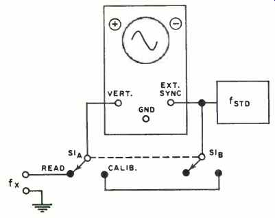
Fig. 1. Suggested switching arrangement and equipment hookup.
Fig. 1 illustrates the basic equipment connections and a suggested switching arrangement. For purposes of this illustration, let us assume we have as a standard a 1000 -cps electronic tuning fork. (Some of these units are of exceptionally high accuracy and stability.) The actual choice of frequency for f_std, will depend on the approximate value of the unknown frequency, f =. Generally, it is desirable that the value of f_std be much greater than that of f.
Notice that the drawing of the oscilloscope includes the two symbols " +" and "-". These may be painted on the scope case if one wishes, or they may be marked on a piece of masking tape or gummed label and merely stuck in the indicated places; the "+" to the left side of the CRT, the "-" to the right side. Their use is in making the determination of whether the derived difference in frequency is additive or subtractive. The function of S1 is to switch the Y-axis or vertical input between the known (standard) and unknown sources.
The stop watch should, preferably, be one that is calibrated in hundredths of a second. This is not mandatory, but the use of such a watch reduces the likelihood of introducing counting or calculating errors.
Measurement Procedure
With the oscilloscope connected as shown and warmed up, check that the following conditions also obtain: The external sync pot is at a neutral (zero) position; that is, no sync is applied. The sweep frequency controls are set to the appropriate range for displaying the unknown frequency. The brightness, focus, and gain controls are set to give a good image. The image should be positioned so that it is totally visible and centered approximately on the center line of the CRT face. This being done, the actual measurement procedure is as follows:
Step 1. Place S1 in the "Read" position. The unknown frequency is now deflecting the scope trace. No sync voltage is applied. By adjusting the coarse and fine sweep-speed controls, obtain a single cycle of the unknown frequency on the CRT (see Fig. 2A) . Carefully adjust the fine frequency control pot to make the single cycle hold stationary, or as nearly so as is possible. Do not use sync. (This step is only to determine which fraction of f.,,, is involved.)
Step 2. Place Si in the "Calibrate" position. It is unlikely that a stationary pattern will be obtained. (If this pattern is stationary, check to see that the sync control has not been turned off the neutral spot.) Cautiously readjust the fine sweep-control pot up or down in frequency, depending on which direction gives the shortest route to obtaining a stationary pattern. (Hint: If the pattern drift is left, or toward the "+" side, slowly turn the pot clockwise to arrest the pattern. If drift is to the right, turn slowly counterclockwise.) When the pattern consists of some whole number of sine waves ( say 3, 5, or 8) , first attempt to stabilize the pattern by carefully adjusting the fine sweep speed. Then carefully inject the sync signal, via the "Ext. Sync" control, so that the pattern is firmly locked. At this point the sweep rate is being accurately controlled by the standard frequency.
Step 3. Suppose that the pattern obtained in this manner consists of 8 sine waves. Note: It will be necessary to allow for a missing portion of the last cycle, due to flyback time.
See Fig. 2B. The exact sweep speed is now the frequency of the standard being used (1000 cps in this case) divided by the number of cycles seen, or 1000/8 = 125.00 cps.
Step 4. Return S1 to "Read" position. Observe the direction of trace movement, but do not touch any controls. On a sheet of paper, record the sign " +" if the pattern drift is left (Fig. 2C), or " " if it is right. This is the sign of the correction to be applied to the last calculation.
Step 5. Immediately begin the timing operation. If the CRT has a transparent scale, or graticule, refer to it. If not, mark with grease pencil some portion of the CRT face through which a part of the trace is drifting. (See Fig. 2D.) This is the reference mark, or index. As each succeeding wave passes through this index, it will be counted.
The technique of timing and counting is very important and, if not properly clone, can be a source of error. Be sure that the first counting utterance is "zero" and not "one." After observing the pattern drift long enough to pick up the rhythm of the trace movement, begin the timing. At the same instant the selected portion of the wave passes through the index, start the stop watch and simultaneously count "zero (the watch is started) , one, two, three ... etc." The greater the number of cycles counted, the more accurate is the result.
For very slow drifts, or beats, a count of from 10 to 20 may be sufficient. For faster ones, it is advisable to count a minimum of 50 to 100. When a sufficient number has been counted, stop the watch. Example: " ... 48, 49, mark!" The watch is stopped at "mark," or 50. All is now done except the calculation. Recall that the sign of the correction was established from the prior observation of drift movement in Step 4. The amount of the correction is calculated as follows: Assume that 50 cycles were counted, and the stop watch recorded 21.42 seconds. This is equivalent to 50/21.42 =2.334 cps. Assuming that in Step 4 an additive correction was indicated, then 125.00 (exact sweep speed) + 2.334 (difference frequency) = 127.334 cps, which is the actual value of the previously unknown frequency f. Depending on the skill with which the timing is performed, the figure in the hundredths place is of questionable accuracy.
(The figure in the thousandths position is only a division result, and has little significance.) An average of three to five runs should enable the actual value of that decimal to be determined with reasonable accuracy. Recall, too, that any timing error becomes smaller the more beats that are counted.
Whatever the error may be, it is divided by the total count taken, just prior to the final calculation.
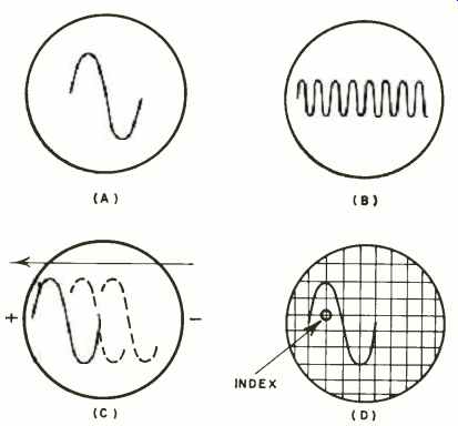
Fig. 2. Waveforms obtained during the measurement procedure.
Discussion of the Technique
All of the foregoing instructions are theoretically sound and practical. If, however, one is restricted to a single, or even two sources for f_std, it will not be long before some inherent limitations will make themselves known. The technique has been presented in its simplest form. To make clear what kind of pattern is a desired indication, only a sinusoidal presentation has been described, as it is the most easily recognized. The patterns obtained in Step 2 are the simplest derivatives of f.,,, that is, they are f /2, f /3, ... f /8, etc. Drift rates faster than about 6 cps are quite difficult to time, by eye. Thus, strict adherence to the patterns described would permit readouts of ± about 6 cycles, of the frequency f /n.
Happily, these limitations have several solutions. Some of these do not involve a departure from the principles of economy that make this measurement technique available to the average reader. And, in any case, the limitations should not detract from the fundamental excellence of the general method. These solutions take the following form: (1) providing additional satisfactory sources of f_std and (2) providing ways to count the more rapidly drifting beat pattern.
A very simple way to get more mileage from a given standard frequency is illustrated. Suppose that, for example, the unknown frequency is 259.00 cps. Using the same 1000-cps standard, it is obvious by inspection that the nearest fraction giving a sine -wave pattern is f /4, or 250.00 cps. However, it is also obvious that this choice will give a 9-cps drift. It is a rare individual who can count at the rate of 9 per second. But if we notice that this rapid drift is occurring, we can go back to Step 1, and instead of selecting one cycle, we can pick one -half cycle. Going to Step 2 will reveal that the nearest pattern is 1/8, or 125.00 cps. The drift rate is going to be (259/2) 125 cps, or 1295 -125.0 =4.5 cps. This rate is easily counted.
One merely remembers to convert the final frequency back to the correct range by multiplying by the same factor used to obtain the desired patterns; in this case, a multiplication by two.
If one wishes to use Lissajous figures, the usefulness of a single standard frequency is greatly extended. Such patterns (ratios) as 5:3, 5:4, 6:5, can provide additional known fractional values of the standard, to overcome the difficulties of rapid drift.
Perhaps an even better way, short of going into more sophisticated and complex aggregations of equipment, is to employ an auxiliary audio-frequency oscillator. If this oscillator is known to have excellent short-term stability, it can be employed with satisfactory results in place of the WWV tones or the accurate tuning fork. The continuously variable feature of the audio oscillator offers the tremendous advantage of furnishing many basic values for the standard frequency. Of course it is necessary to synchronize, or compare, the oscillator with a known standard, just before making a measurement, and proceed directly to make the measurement. Dial readings are valueless and not used except possibly as guides, say, for the 100-cycle dial increments. The actual oscillator setting, if used as a standard, must in every instance be derived by comparison with a standard, just before use.