1. Psychoacoustics and Subjective Quantities
Unlike other senses, it is surprising how limited our vocabulary is when talking about hearing.
Especially in the audio industry, we do not often discriminate between subjective and objective quantities. For instance, the quantities of frequency, level, spectrum, etc. are all objective, in a sense that they can be measured with a meter or an electronic device; whereas the concepts of pitch, loudness, timbre, etc. are subjective, and they are auditory perceptions in our heads. Psycho acoustics investigates these subjective quantities (i.e., our perception of hearing), and their relationship with the objective quantities in acoustics. Psychoacoustics got its name from a field within psychology--i.e., recognition science-which deals with all kinds of human perceptions, and it is an interdisciplinary field of many areas, including psychology, acoustics, electronic engineering, physics, biology, physiology, computer science, etc.
Although there are clear and strong relationships between certain subjective and objective quantities--e.g., pitch versus frequency-other objective quantities also have influences. For example, changes in sound level can affect pitch perception. Furthermore, because no two persons are identical, when dealing with perceptions as in psychoacoustics, there are large individual differences, which can be critical in areas such as sound localization.
In psychoacoustics, researchers have to consider both average performances among population and individual variations. Therefore, psychophysical experiments and statistical methods are widely used in this field.
Compared with other fields in acoustics, psychoacoustics is relatively new, and has been developing greatly. Although many of the effects have been known for some time (e.g., Hass effect), new discoveries have been found continuously. To account for these effects, models have been proposed. New experimental findings might invalidate or modify old models or make certain models more or less popular. This process is just one representation of how we develop our knowledge. For the purpose of this handbook, we will focus on summarizing the known psychoacoustic effects rather than discussing the developing models.
2. Ear Anatomy and Function
Before discussing various psychoacoustic effects, it is necessary to introduce the physiological bases of those effects, namely the structure and function of our auditory system. The human ear is commonly considered in three parts: the outer ear, the middle ear, and the inner ear. The sound is gathered (and as we shall see later, modified) by the external ear called the pinna and directed down the ear canal (auditory meatus). This canal is terminated by the tympanic membrane (ear drum). These parts constitute the outer ear, as shown in FIGs. 1 and 2. The other side of the eardrum faces the middle ear. The middle ear is air filled, and pressure equalization takes place through the eustachian tube opening into the pharynx so normal atmospheric pres sure is maintained on both sides of the eardrum. Fastened to the eardrum is one of the three ossicles, the malleus which, in turn, is connected to the incus and stapes. Through the rocking action of these three tiny bones the vibrations of the eardrum are transmitted to the oval window of the cochlea with admirable efficiency. The sound pressure in the liquid of the cochlea is increased some 30-40 dB over the air pressure acting on the eardrum through the mechanical action of this remarkable middle ear system. The clear liquid filling the cochlea is incompressible, like water. The round window is a relatively flexible pressure release allowing sound energy to be transmitted to the fluid of the cochlea via the oval window. In the inner ear the traveling waves set up on the basilar membrane by vibrations of the oval window stimulate hair cells that send nerve impulses to the brain.
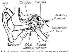
FIG. 1. A cross-section of the human ear showing the relationship of the
various parts. Pinna; Ossicles; Cochlea; Auditory nerve; Eustachian tube; Round
window; Oval window; Eardrum
2.1 Pinna
The pinna, or the human auricle, is the most lateral (i.e., outside) portion of our auditory system. The beauty of these flaps on either side of our head may be questioned, but not the importance of the acoustical function they serve. FIG. 3 shows an illustration of various parts of the human pinna. The entrance to the ear canal, or concha, is most important acoustically for filtering because it contains the largest air volume in a pinna. Let us assume for the moment that we have no pinnae, just holes in the head, which is actually a simplest model for human hearing, called the spherical head model. Cup ping our hands around the holes would make sounds louder as more sound energy is directed into the opening. How much does the pinna help in directing sound energy into the ear canal? We can get some idea of this by measuring the sound pressure at the opening of the ear canal with and without the hand behind the ear. Wiener and Ross did this and found a gain of 3 to 5 dB at most frequencies, but a peak of about 20 dB in the vicinity of 1500 Hz. FIG. 4 shows the transfer function measured by Shaw,5 and the curves numbered 3 and 4 are for concha and pinna flange, respectively. The irregular and asymmetric shape of a pinna is not just for aesthetic reasons. In Section 3.11, we will see that it is actually important for our ability to localize sounds and to aid in spatial-filtering of unwanted conversations.
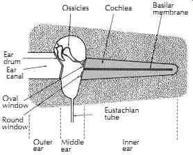
FIG. 2. Highly idealized portrayal of the outer ear, middle ear, and inner
ear. Ossicles, Cochlea, Basilar membrane, Ear drum, Ear canal, Oval window,
Round window, Outer ear, Middle ear, Eustachian tube, Inner ear
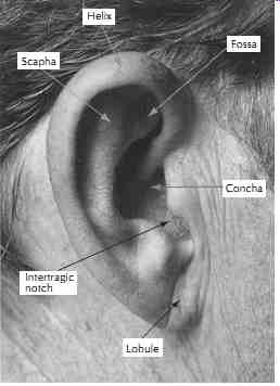
FIG. 3. The human outer ear, the pinna, with identification of some of the
folds, cavities, and ridges that have significant acoustical effect.
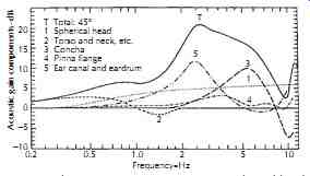
FIG. 4. The average pressure gain contributed by the different components
of the outer ear in humans. The sound source is in the horizontal plane, 45-deg.
from straight ahead. (After Shaw, Reference 5.) Scapha Helix Fossa Concha Lobule
Intertragic notch T Total: 45 degree 1 Spherical head 2 Torso and neck, etc.
3 Concha; 4 Pinna flange; 5 Ear canal and eardrum; Frequency-Hz; Acoustic gain
components-dB
2.2 Temporal Bones
On each of the left and right sides of our skull, behind the pinna, there is a thin, fanlike bone-namely, the temporal bone-covering the entire human ear, except for the pinna. This bone can be further divided into four portions--i.e., the squamous, mastoid, tympanic and petrous portions. The obvious function for the temporal bone is to protect our auditory system. Other than cochlear implant patients, whose temporal bone has to be partly removed during a surgery, people might not pay much attention to it, especially regarding acoustics.
However the sound energy that propagates through the bone into our inner ear, as opposed to through the ear canal and middle ear, is actually fairly significant. For patients with conductive hearing loss--e.g., damage of middle ear-there are currently commercially available devices, which look something like headphones and are placed on the temporal bone. People with normal hearing can test it by plugging their ears while wearing the device. Although the timbres sound quite different from normal hearing, the filtered speech is clear enough to understand. Also because of this bone conduction, along with other effects such as acoustic reflex, one hears his or her own voice differently from how other people hear the voice.
While not receiving much attention in everyday life, it might be sometimes very important. For example, an experienced voice teacher often asks a student singer to record his or her own singing and playback with an audio system. The recording will sound unnatural to the singer but will be a more accurate representation of what the audience hears.
2.3 Ear Canal
The ear canal has a diameter about 5 to 9 mm and is about 2.5 cm long. It is open to the outside environment at the concha, and is closed at the tympanic membrane.
Acoustically, it can be considered as a closed pipe whose cross-sectional shape and area vary along its length. Although being bended and irregular in shape, the ear canal does demonstrate the modal characteristic of a closed pipe. It has a fundamental frequency of about 3 kHz, corresponding to a quarter wavelength close to the length of the ear canal. Because of this resonant frequency, our hearing is most sensitive to a frequency band around 3 kHz, which is, not just by coincidence, the most important frequency band of human speech. On FIG. 4, the number 5 curve shows the effect of the ear canal, taking the eardrum into account as well. As can be seen, there is an approximately 11 dB of gain at around 2.5 kHz. After combining all the effects of head, torso and neck, pinna, ear canal and eardrum, the total transfer function is the curve marked with a letter T on FIG. 4. It is relatively broadly tuned between 2 and 7 kHz, with as much as 20 dB of gain. Unfortunately, because of this resonance, in very loud noisy environments with broadband sound, hearing damage usually first happens around 4 kHz.
2.4 Middle Ear
The outer ear, including the pinna and the ear canal, ends at the eardrum. It is an air environment with low impedance. On the other hand, the inner ear, where the sensory cells are, is a fluid environment with high impedance. When sound (or any wave) travels from one medium to another, if the impedances of the two media do not match, much of the energy would be reflected at the surface, without propagating into the second medium. For the same reason, we use microphones to record in the air and hydrophones to record under water.
To make our auditory system efficient, the most important function of the middle ear is to match the impedances of outer and inner ears. Without the middle ear, we would suffer a hearing loss of about 30 dB (by mechanical analysis and experiments on cats).
A healthy middle ear (without middle ear infection) is an air-filled space. When swallowing, the eustachian tube is open to balance the air pressure inside the middle ear and that of the outside world. Most of the time, however, the middle ear is sealed from the outside environment. The main components of the middle ear are the three ossicles, which are the smallest bones in our body: the malleus, incus, and stapes. These ossicles form an ossiclar chain, which is firmly fixed on the eardrum and the oval window on each side. Through mostly three types of mechanical motions-namely piston motion, lever motion and buckling motion8-the acoustic energy is transferred into the inner ear effectively. The middle ear can be damaged temporarily by middle ear infection, or permanently by genetic disease. Fortunately, with current technology, doctors can rebuild the ossicles with titanium, the result being a total recovering of hearing. Alternatively one can use devices that rely on bone conduction.
2.4.1 Acoustic Reflex
There are two muscles in the middle ear: the tensor tympani that is attached to the malleus, and the stapedius muscle that is attached to the stapes. Unlike other muscles in our bodies, these muscles form an angle with respect to the bone, instead of along the bone, which makes them very ineffective for motion. Actually the function of these muscles is for changing the stiffness of the ossicular chain. When we hear a very loud sound--i.e., at least 75 dB higher than the hearing threshold-when we talk or sing, when the head is touched, or when the body moves, these middle ear muscles will contract to increase the stiffness of the ossicular chain, which makes it less effective, so that our inner ear is protected from exposure to the loud sound. However, because this process involves a higher stage of signal processing, and because of the filtering features, this protection works only for slow onset and low-frequency sound (up to 1.2 kHz12) and is not effective for noises such as an impulse or noise with high frequencies (e.g., most of the music recordings today).
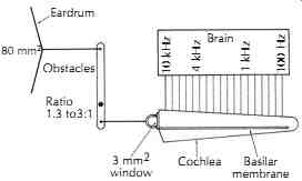
FIG. 5. The mechanical system of the middle ear.
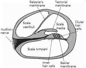
FIG. 6. Cross-sectional sketch of the cochlea.
Eardrum 80 mm^2 Obstacles Ratio 1.3 to 3:1 3 mm^2 window Cochlea Basilar membrane Brain 10 kHz 4 kHz 1 kHz 100 Hz; Auditory nerve; Reissner's membrane; Tectorial membrane; Outer hair cells; Basilar membrane; Inner hair cells; Scala vestibule; Scala tympani; Scala media
2.5 Inner Ear
The inner ear, or the labyrinth, is composed of two systems: the vestibular system, which is critical to our sense of balance, and the auditory system which is used for hearing. The two systems share fluid, which is separated from the air-filled space in the middle ear by the oval window and the round window. The auditory portion of the inner ear is the snail-shaped cochlea. It is a mechanical-to-electrical transducer and a frequency-selective analyzer, sending coded nerve impulses to the brain. This is represented crudely in FIG. 5. A rough sketch of the cross section of the cochlea is shown in FIG. 6. The cochlea, throughout its length (about 35 mm if stretched out straight), is divided by Reissner's membrane and the basilar membrane into three separate compartments-namely, the scala vestibuli, the scala media, and the scala tympani. The scala vestibuli and the scala tympani share the same fluid, perilymph, through a small hole, the helicotrema, at the apex; while the scala media contains another fluid, endolymph, which contains higher density of potassium ions facilitating the function of the hair cells. The basilar membrane supports the Organ of Corti, which contains the hair cells that convert the relative motion between the basilar membrane and the tectorial membrane into nerve pulses to the auditory nerve.
When an incident sound arrives at the inner ear, the vibration of the stapes is transported into the scala vestibuli through the oval window. Because the cochlear fluid is incompressible, the round window connected to the scala tympani vibrates accordingly. Thus, the vibration starts from the base of the cochlea, travels along the scala vestimbuli, all the way to the apex, and then through the helicotrema into the scala tympani, back to the base, and eventually ends at the round window. This establishes a traveling wave on the basilar membrane for frequency analysis. Each location at the basilar membrane is most sensitive to a particular frequency--i.e., the characteristic frequency-although it also responds to a relatively broad frequency band at smaller amplitude. The basilar membrane is narrower (0.04 mm) and stiffer near the base, and wider (0.5 mm) and looser near the apex. (By contrast, when observed from outside, the cochlea is wider at the base and smaller at the apex.) Therefore, the characteristic frequency decreases gradually and monotonically from the base to the apex, as indicated in FIG. 5. The traveling-wave phenomenon illustrated in FIGs. 7 and 8 shows the vibration patterns--i.e., amplitude versus location-for incident pure tones of different frequencies. An interesting point in FIG. 8 is that the vibration pattern is asymmetric, with a slow tail close to the base (for high frequencies) and a steep edge close to the apex (for low frequencies). Because of this asymmetry, it is easier for the low frequencies to mask the high frequencies than vice versa.
Within the Organ of Corti on the basilar membrane, there are a row of inner hair cells (IHC), and three to five rows of outer hair cells (OHC), depending on location. There are about 1500 IHCs and about 3500 OHCs.
Each hair cell contains stereociliae (hairs) that vibrate corresponding to the mechanical vibration in the fluid around them. Because each location on the basilar membrane is most sensitive to its own characteristic frequency, the hair cells at the location also respond most to its characteristic frequency. The IHCs are sensory cells, like microphones, which convert mechanical vibration into electrical signal--i.e., neural firings.
The OHCs, on the other hand, change their shapes according to the control signal received from efferent nerves. Their function is to give an extra gain or attenuation, so that the output of the IHC is tuned to the characteristic frequency much more sharply than the IHC itself. FIG. 9 shows the tuning curve (output level vs. frequency) for a particular location on the basilar membrane with and without functioning OHCs. The tuning curve is much broader with poor frequency selectivity when the OHCs do not function. The OHCs make our auditory system an active device, instead of a passive microphone. Because the OHCs are active and consume a lot of energy and nutrition, they are usually damaged first due to loud sound or ototoxic medicines (i.e., medicine that is harmful to the auditory system).
Not only does this kind of hearing loss make our hearing less sensitive, it also makes our hearing less sharp. Thus, as is easily confirmed with hearing-loss patients, simply adding an extra gain with hearing aids would not totally solve the problem.
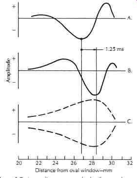
FIG. 7. A traveling wave on the basilar membrane of the inner ear. (After
von Békésy, Reference 13.) The exaggerated amplitude of the basilar membrane
for a 200 Hz wave traveling from left to right is shown at A. The same wave
1.25 ms later is shown at B. These traveling 200 Hz waves all fall within the
envelope at C.
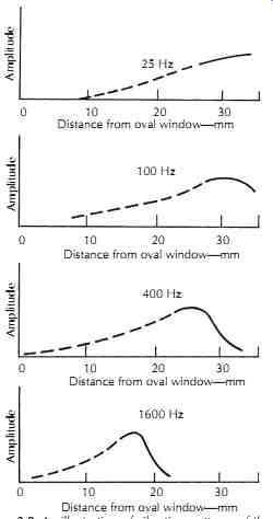
FIG. 8. An illustration of vibration patterns of the hair cells on the basilar
membrane for various incident pure tones. There is a localized peak response
for each audible frequency. (After von Békésy, Reference 13.) Distance from
oval window}mm
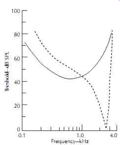
FIG. 9. Tuning curve with (solid) and without (dashed) functioning outer
hair cells. (Liberman and Dodds, Reference 14.)
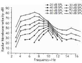
FIG. 10. Tuning curve at various levels at a particular location of the basilar
membrane of a chinchilla. (Plack, Reference 15, p90, Ruggero et al., Reference
16.)
3. Frequency Selectivity
3.1 Frequency Tuning
As discussed in Section 3, the inner hair cells are sharply tuned to the characteristic frequencies with help from the outer hair cells. This tuning character is also conserved by the auditory neurons connecting to the inner hair cells. However, this tuning feature varies with level. FIG. 10 shows a characteristic diagram of tuning curves from a particular location on the basilar membrane at various levels. As can be seen in this graph, as level increases, the tuning curve becomes broader, indicating less frequency selectivity. Thus, in order to hear music more sharply, one should play back at a relatively low level. Moreover, above 60 dB, as level increases, the characteristic frequency decreases. Therefore when one hears a tone at a high level, a neuron that is normally tuned at a higher characteristic frequency is now best tuned to the tone. Because eventually the brain perceives pitch based on neuron input, at high levels, with out knowing that the characteristic frequency has decreased, the brain hears the pitch to be sharp.
Armed with this knowledge, one would think that someone who was engaged in critical listening-a recording engineer, for example-would choose to listen at moderate to low levels. Why then do so many audio professionals choose to monitor at very high levels? There could be many reasons. Loud levels may be more exciting. It may simply be a matter of habit.
For instance, an audio engineer normally turns the volume to his or her customary level fairly accurately.
Moreover, because frequency selectivity is different at different levels, an audio engineer might choose to make a recording while listening at a "realistic" or "performance" level rather than monitoring at a level that is demonstratedly more accurate. Finally, of course, there are some audio professionals who have lost some hearing already, and in order to pick up certain frequency bands they keep on boosting the level, which unfortunately further damages their hearing.
3.2 Masking and Its Application in Audio Encoding
Suppose a listener can barely hear a given acoustical signal under quiet conditions. When the signal is playing in presence of another sound (called "a masker"), the signal usually has to be stronger so that the listener can hear it. The masker does not have to include the frequency components of the original signal for the masking effect to take place, and a masked signal can already be heard when it is still weaker than the masker.
Masking can happen when a signal and a masker are played simultaneously (simultaneous masking), but it can also happen when a masker starts and ends before a signal is played. This is known as forward masking.
Although it is hard to believe, masking can also happen when a masker starts after a signal stops playing! In general, the effect of this backward masking is much weaker than forward masking. Forward masking can happen even when the signal starts more than 100 ms after the masker stops, but backward masking disappears when the masker starts 20 ms after the signal.
The masking effect has been widely used in psycho acoustical research. For example, FIG. 10 shows the tuning curve for a chinchilla. For safety reasons, performing such experiments on human subjects is not permitted. However, with masking effect, one can vary the level of a masker, measure the threshold (i.e., the minimum sound that the listener can hear), and create a diagram of a psychophysical tuning curve that reveals similar features.
Besides scientific research, masking effects are also widely used in areas such as audio encoding. Now, with distribution of digital recordings, it is desirable to reduce the sizes of audio files. There are lossless encoders, which is an algorithm to encode the audio file into a smaller file that can be completely reconstructed with another algorithm (decoder). However, the file sizes of the lossless encoders are still relatively large.
To further reduce the size, some less important information has to be eliminated. For example, one might eliminate high frequencies, which is not too bad for speech communication. However, for music, some important quality might be lost. Fortunately, because of the masking effect, one can eliminate some weak sounds that are masked so that listeners hardly notice the difference. This technique has been widely used in audio encoders, such as MP3.
3.3 Auditory Filters and Critical Bands
Experiments show that our ability to detect a signal depends on the bandwidth of the signal. Fletcher (1940) found that, when playing a tone in the presence of a bandpass masker, as the masker bandwidth was increased while keeping the overall level of the masker unchanged, the threshold increased as bandwidth increased up to a certain limit, beyond which the thresh old remained constant. One can easily confirm that, when listening to a bandpass noise with broadening bandwidth and constant overall level, the loudness is unchanged, until a certain bandwidth is reached, and beyond that bandwidth the loudness increases as band width increases, although the reading of an SPL meter is constant. An explanation to account for these effects is the concept of auditory filters. Fletcher proposed that, instead of directly listening to each hair cell, we hear through a set of auditory filters, whose center frequencies can vary or overlap, and whose bandwidth is varying according to the center frequency. These bands are referred to as critical bands (CB). Since then, the shape and bandwidth of the auditory filters have been care fully studied. Because the shape of the auditory filters is not simply rectangular, it is more convenient to use the equivalent rectangular bandwidth (ERB), which is the bandwidth of a rectangular filter that gives the same transmission power as the actual auditory filter. Recent study by Glasberg and Moore (1990) gives a formula for ERB for young listeners with normal hearing under moderate sound pressure levels21: where, the center frequency of the filter F is in kHz, ERB is in Hz.
Sometimes, it is more convenient to use an ERB number as in Eq. 1, similar to the Bark scale proposed by Zwicker et al.
... where, the center frequency of the filter F is in kHz.
Table 1 shows the ERB and Bark scale as a function of the center frequency of the auditory filter.
The Bark scale is also listed as a percentage of center frequency, which can then be compared to filters commonly used in acoustical measurements: octave (70.7%), half octave (34.8%), one-third octave (23.2%), and one-sixth octave (11.6%) filters. The ERB is shown in FIG. 11 as a function of frequency. One-third octave filters which are popular in audio and have been widely used in acoustical measurements ultimately have their roots in the study of human auditory response.
However, as FIG. 11 shows, the ERB is wider than octave for frequencies below 200 Hz; is smaller than octave for frequencies above 200 Hz; and, above 1 kHz, it approaches octave.

Table 1. Critical Bandwidths of the Human Ear
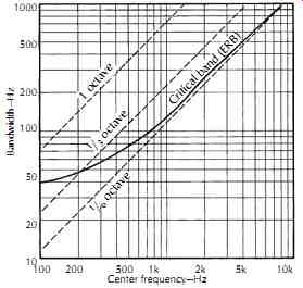
FIG. 11. A plot of critical bandwidths (calculated ERBs) of the human auditory
system compared to constant percentage bandwidths of filter sets commonly used
in acoustical measurements.
4. Nonlinearity of the Ear
When a set of frequencies are input into a linear system, the output will contain only the same set of frequencies, although the relative amplitudes and phases can be adjusted due to filtering. However, for a nonlinear system, the output will include new frequencies that are not present in the input. Because our auditory system has developed mechanisms such as acoustic reflex in the middle ear and the active processes in the inner ear, it is nonlinear. There are two types of nonlinearity-namely, harmonic distortion and combination tones. Harmonic distortion can be easily achieved by simply distorting a sine-tone. The added new components are harmonics of the original signal. A combination tone happens when there are at least two frequencies in the input. The output might include combination tones according to (eqn. 2) where, fc is the frequency of a combination tone, f1 and f2 are the two input frequencies, and n and m are any integer numbers.
For example, when two tones at 600 and 700 Hz are input, the output might have frequencies such as 100 Hz (= 700 _ 600 Hz), 500 Hz (= 2 × 600 _ 700 Hz), and 400 Hz (= 3 × 600 _ 2 × 700 Hz), etc.
Because the harmonic distortion does not change the perception of pitch, it would not be surprising if we are less tolerant of the combination tones.
Furthermore, because the auditory system is active, even in a completely quiet environment, the inner ear might generate tones. These otoacoustic emissions are a sign of a healthy and functioning inner ear, and quite different from the tinnitus resulting from exposure to dangerously high sound pressure levels.
5. Perception of Phase
The complete description of a given sound includes both an amplitude spectrum and a phase spectrum.
People normally pay a lot of attention to the amplitude spectrum, while caring less for the phase spectrum. Yet academic researchers, hi-fi enthusiasts, and audio engineers all have asked, "Is the ear able to detect phase differences?" About the middle of the last century, G. S. Ohm wrote, "Aural perception depends only on the amplitude spectrum of a sound and is independent of the phase angles of the various components contained in the spectrum." Many apparent confirmations of Ohm's law of acoustics have later been traced to crude measuring techniques and equipment.
Actually, the phase spectrum sometimes can be very important for the perception of timbre. For example, an impulse and white noise sound quite different, but they have identical amplitude spectrum. The only difference occurs in the phase spectrum. Another common example is speech: if one scrambles the relative phases in the spectrum of a speech signal, it will not be intelligible. Now, with experimental evidence, we can confirm that our ear is capable of detecting phase information. For example, the neural firing of the auditory nerve happens at a certain phase, which is called the phase-locking, up to about 5 kHz.
The phase-locking is important for pitch perception. In the brainstem, the information from left and right ears is integrated, and the interaural phase difference can be detected, which is important for spatial hearing. These phenomena will be discussed in more detail in Sections 3.9 and 3.11.
6. Auditory Area and Thresholds
The auditory area depicted in FIG. 12 describes, in a technical sense, the limits of our aural perception. This area is bounded at low sound levels by our threshold of hearing. The softest sounds that can be heard fall on the threshold of hearing curve. Above this line the air molecule movement is sufficient to elicit a response. If, at any given frequency, the sound pressure level is increased sufficiently, a point is reached at which a tick ling sensation is felt in the ears. If the level is increased substantially above this threshold of feeling, it becomes painful. These are the lower and upper boundaries of the auditory area. There are also frequency limitations below about 20 Hz and above about 16 kHz, limitations that (like the two thresholds) vary considerably from individual to individual. We are less concerned here about specific numbers than we are about principles. On the auditory area of FIG. 12, all the sounds of life are played out-low frequency or high, very soft or very intense. Speech does not utilize the entire auditory area.
Its dynamic range and frequency range are quite limited. Music has both a greater dynamic range than speech and a greater frequency range. But even music does not utilize the entire auditory area.
7. Hearing Over Time
If our ear was like an ideal Fourier analyzer, in order to translate a waveform into a spectrum, the ear would have to integrate over the entire time domain, which is not practical and, of course, not the case. Actually, our ear only integrates over a limited time window (i.e., a filter on the time axis), and thus we can hear changes of pitch, timbre, and dynamics over time, which can be shown on a spectrogram instead of a simple spectrum.
Mathematically, it is a wavelet analysis instead of a Fourier analysis. Experiments on gap detection between tones at different frequencies indicate that our temporal resolution is on the order of 100 ms, which is a good estimate of the time window of our auditory system. For many perspectives (e.g., perceptions on loudness, pitch, timbre), our auditory system integrates acoustical information within this time window.
8. Loudness
Unlike level or intensity, which are physical or objective quantities, loudness is a listener's subjective perception. As the example in Section 3.3, even if the SPL meter reads the same level, a sound with a wider band width might sound much louder than a sound with a smaller bandwidth. Even for a pure tone, although loudness follows somewhat with level, it is actually a quite complicated function, depending on frequency. A tone at 40 dB SPL is not necessarily twice as loud as another sound at 20 dB SPL. Furthermore, loudness also varies among listeners. For example, a listener who has lost some sensitivity in a certain critical band will perceive any signal in that band to be at a lower level relative to someone with normal hearing.
Although there is no meter to directly measure a subjective quantity such as loudness, psycho-physical scaling can be used to investigate loudness across subjects. Subjects can be given matching tasks, where they are asked to adjust the level of signals until they match, or comparative tasks, where they are asked to compare two signals and estimate the scales for loudness.
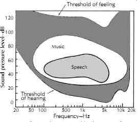
FIG. 12. All sounds perceived by humans of average hearing acuity fall within
the auditory area. This area is defined by the threshold of hearing and the
threshold of feeling (pain) and by the low and high frequency limits of hearing.
Music and speech do not utilize the entire auditory area available, but music
has the greater dynamic range (vertical) and frequency demands (horizontal).
8.1 Equal Loudness Contours and Loudness Level
By conducting experiments using pure tones with a large population, Fletcher and Munson at Bell Labs (1933) derived equal loudness contours, also known as the Fletcher-Munson curves. FIG. 13 shows the equal loudness contours later refined by Robinson and Dadson, which have been recognized as an international standard. On the figure, the points on each curve correspond to pure tones, giving the same loudness to an average listener. For example, a pure tone at 50 Hz at 60 dB SPL is on the same curve as a tone at 1 kHz at 30 dB. This means that these two tones have identical loudness to an average listener. Obviously, the level for the 50 Hz tone is 30 dB higher than the level of the 60 Hz tone, which means that we are much less sensitive to the 50 Hz tone. Based on the equal loudness con tours, loudness level, in phons, is introduced. It is always referenced to a pure tone at 1 kHz. The loudness level of a pure tone (at any frequency) is defined as the level of a 1 kHz tone that has identical loudness to the given tone for an average listener. For the above example, the loudness of the 50 Hz pure tone is 30 phons, which means it is as loud as a 30 dB pure tone at 1 kHz.
The lowest curve marked with "minimum audible" is the hearing threshold. Although many normal listeners can hear tones weaker than this threshold at some frequencies, on average, it is a good estimate of a minimum audible limit. The tones louder than the curve of 120 phons will cause pain and hearing damage.
The equal loudness contours also show that human hearing is most sensitive around 4 kHz (which is where the hearing damage due to loud sounds first happens), less sensitive to high frequencies, and much less sensitive for very low frequencies (which is why a subwoofer has to be very powerful to produce strong bass, the price of which is the masking of mid-and high-frequencies and potential hearing damage). A study of this family of curves tells us why treble and bass frequencies seem to be missing or down in level when favorite recordings are played back at low levels.
One might notice that for high frequencies above 10 kHz, the curves are nonmonotonic for low levels.
This is due to the second resonant mode of the ear canal. Moreover, at low frequencies below 100 Hz, the curves are close to each other, and the change of a few dB can give you the feeling of more than 10 dB of dynamic change at 1 kHz. Furthermore, the curves are much flatter at high levels, which unfortunately encouraged many to listen to reproduced music at abnormally high levels, again causing hearing damage. Actually, even if one wanted to have flat or linear hearing, listening at abnormally high levels might not be wise, because the frequency selectivity of our auditory system will be much poorer, leading to much greater interaction between various frequencies. Of course, one limitation of listening at a lower level is that, if some frequency components fall below the hearing threshold, then they are not audible. This problem is especially important for people who have already lost some acuity at a certain frequency, where his or her hearing threshold is much higher than normal. However, in order to avoid further damage of hearing, and in order to avoid unnecessary masking effect, one still might consider listening at moderate levels.
The loudness level considers the frequency response of our auditory system, and therefore is a better scale than the sound pressure level to account for loudness.
However, just like the sound pressure level is not a scale for loudness, the loudness level does not directly represent loudness, either. It simply references the sound pressure level of pure tones at other frequencies to that of a 1 kHz pure tone. Moreover, the equal loudness contours were achieved with pure tones only, without consideration of the interaction between frequency components--e.g., the compression within each auditory filter. One should be aware of this limit when dealing with broadband signals, such as music.
8.2 Level Measurements with A-, B-, and C-Weightings
Although psycho-acoustical experiments give better results on loudness, practically, level measurement is more convenient. Because the equal loudness contours are flatter at high levels, in order to make level measurements somewhat representing our loudness perception, it is necessary to weight frequencies differently for measurements at different levels. FIG. 14 shows the three widely used weighting functions.
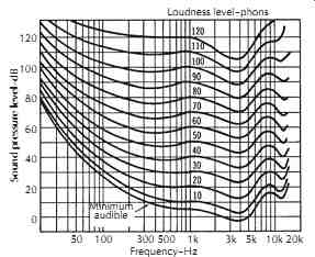
FIG. 13. Equal loudness contours for pure tones in a frontal sound field
for humans of average hearing acuity determined by Robinson and Dadson. The
loudness levels in phons correspond to the sound pressure levels at 1000 Hz.
(ISO Recommendation 226).
The A-weighting level is similar to our hearing at 40 dB, and is used at low levels; the B-weighting level represents our hearing at about 70 dB; and the C-weighting level is more flat, representing our hearing at 100 dB, and thus is used at high levels. For concerns on hearing loss, the A-weighting level is a good indicator, although hearing loss often happens at high levels.
8.3 Loudness in Sones
Our hearing for loudness is definitely a compressed function (less sensitive for higher levels), giving us both sensitivity for weak sounds and large dynamic range for loud sounds. However, unlike the logarithmic scale (dB) that is widely used in sound pressure level, experimental evidence shows that loudness is actually a power law function of intensity and pressure as shown in Eq. 3. where, k and are constants accounting for individuality of listeners, I is the sound intensity, p is the sound pressure, D varies with level and frequency.
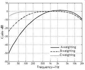
FIG. 14. Levels with A-, B-, and C-weightings. (Reference 27.)
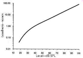
FIG. 15. Comparison between loudness in sones and loudness level in phons
for a 1 kHz tone. (Plack, Reference 15, p118, data from Hellman, Reference
28.)
The unit for loudness is sones. By definition, one sone is the loudness of a 1 kHz tone at a loudness level of 40 phons, the only point where phons and SPL meet.
If another sound sounds twice as loud as the 1 kHz tone at 40 phons, it is classified as 2 sones, etc. The loudness of pure tones in sones is compared with the SPL in dB in FIG. 15. The figure shows that above 40 dB, the curve is a straight line, corresponding to an exponent of about 0.3 for sound intensity and an exponent of 0.6 for sound pressure as in Eq. 3. The exponent is much greater for levels below 40 dB, and for frequencies below 200 Hz (which can be confirmed by the fact that the equal loudness contours are compact for frequencies below 200 Hz on FIG. 13).
One should note that Eq. 3-3 holds for not only pure tones, but also bandpass signals within an auditory filter (critical band). The exponent of 0.3 (<1) indicates compression within the filter. However, for a broad band signal that is wider than one critical bandwidth, Eq. 3 holds for each critical band, and the total loudness is simply the sum of loudness in each band (with no compression across critical bands).
8.4 Loudness versus Bandwidth
Due to less compression across critical bands, broad band sounds, such as a rocket launching or a jet aircraft taking off, seem to be much louder than pure tones or narrow bands of noise of the same sound pressure level.
In fact, increasing the bandwidth does not increase loudness until the critical bandwidth is exceeded. Beyond that point multiple critical bands are excited, and the loudness increases markedly with increase in bandwidth because of less compression across critical bands. For this reason, the computation of loudness for a wide band sound must be based on spectral distribution of energy. Filters no narrower than critical bands are required and octave filters are commonly used.
8.5 Loudness of Impulses
Life is filled with impulse-type sounds: snaps, pops, crackles, bangs, bumps, and rattles. For impulses or tone bursts with duration greater than 100 ms, loudness is independent of pulse width. The effect on loudness for pulses shorter than 200 ms is shown in FIG. 16.
This curve shows how much higher the level of short pulses of noise and pure tones must be to sound as loud as continuous noise or pure tones. Pulses longer than 200 ms are perceived to be as loud as continuous noise or tones of the same level. For the shorter pulses, the pulse level must be increased to maintain the same loudness as for the longer pulses. Noise and tonal pulses are similar in the level of increase required to maintain the same loudness. FIG. 16 indicates that the ear has a time constant of about 200 ms, confirming the time window on the order of 100 ms, as discussed in Section 3.7. This means that band levels should be measured with RMS detectors having integration times of about 200 ms. This corresponds to the FAST setting on a sound level meter while the SLOW setting corresponds to an integration time of 500 ms.
8.6 Perception of Dynamic Changes
How sensitive is our hearing of dynamic changes? In other words, how much intensity or level change will lead to a perception of change of loudness? To discuss this kind of problem, we need the concept of just-noticeable difference (JND), which is defined as the minimum change that can be detected. Weber's Law states that the JND in intensity, in general and not necessarily for hearing, is proportional to the overall intensity. If Weber's Law holds, the Weber fraction in dB as defined in Eq. 4 would be a constant, independent of the overall intensity and the overall level.
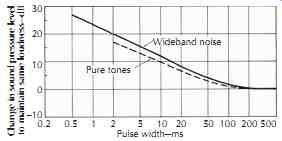
FIG. 16. Short pulses of sound must be increased in level to sound as loud
as longer pulses.
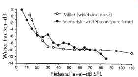
FIG. 17 shows the measurement of the Weber fraction for broadband signals
up to 110 dB SPL.
Above 30 dB, the Weber fraction in dB is indeed a constant of about _10 dB, corresponding to a JND ('L) of 0.4 dB.
However, for weak sounds below 30 dB, the Weber fraction in dB is higher, and can be as high as 0 dB, corresponding to a JND ('L) of 3 dB. In other words, our hearing is less sensitive (in level) for dynamic changes of sounds weaker than 30 dB. Interestingly, when measuring with pure tones, it was found that the Weber fraction is slightly different from the broadband signals. This phenomenon is known as the near-miss Weber's Law. FIG. 17 includes a more recent measurement for pure tones, 31 which demonstrates that the Weber fraction gradually decreases up to 85 dB SPL and can be lower than _12 dB, corresponding to a JND ('L) less than 0.3 dB. The near-miss Weber's Law for pure tones is believed to be associated with the broad excitation patterns across frequency at high levels.
FIG. 17. Just-noticeable difference (JND) for a broad band noise and for
a 1 kHz tone. (After Plack, Reference 15; data from Miller, Reference 29, and
Viemeister and Bacon, Reference 31.) Pedestal level-dB SPL Weber fraction-dB
Miller (wideband noise) Viemeister and Bacon (pure tone)
Next >>