|
|
3.5 Preparation
There are many measurements that can be performed on a sound system. A prerequisite to any measurement is to answer the following questions:
1. What am I trying to measure?
2. Why am I trying to measure it?
3. Is it audible?
4. Is it relevant?
Failure to consider these questions can lead to hours of wasted time and a hard drive full of meaningless data. Even with the incredible technologies that we have available to us, the first part of any measurement session is to listen. It can take many hours to determine what needs to be measured to solve a sound system problem, yet the actual measurement itself can often be completed in seconds. Using an analogy from the medical field, the physician must query the patient at length to narrow down the ailment. The more that is known about the ailment, the more specific and relevant the tests that can be run for diagnosis. There is no need to test for tonsillitis if the problem is a sore back!
1. What am I measuring? A fundamental decision that precedes a meaningful measurement is how much of the room's response to include in the measured data. Modern measurement systems have the ability to perform semi-anechoic measurements, and the measurer must decide if the loudspeaker, the room, or the combination needs to be measured. If one is diagnosing loudspeaker ailments, there is little reason to select a time window long enough to include the effects of late reflections and reverberation. A properly selected time window can isolate the direct field of the loudspeaker and allow its response to be evaluated independently of the room.
If one is trying to measure the total decay time of the room, the direct sound field becomes less important, and a microphone placement and time window are selected to capture the entire energy decay. Most modern measurement systems acquire the complete impulse response, including the room decay, so the choice of the time window size can be made after the fact during post processing.
2. Why am I measuring? There are several reasons for performing acoustic measurements in a space. An important reason for the system designer is to characterize the listening environment. Is it dead? Is it live? Is it reverberant? These questions must be considered prior to the design of a sound system for the space. While the human hearing system can provide the answers to these questions, it cannot document them and it is easily deceived. Measurements might also be performed to document the performance of an existing system prior to performing changes or adding room treatment.
Customers sometimes forget how bad it once sounded after a new or upgraded system is in place for a few weeks.
The most common reason for performing measurements on a system is for calibration purposes. This can include equalization, signal alignment, crossover selection, and a multiplicity of other reasons. Since loudspeakers interact in a complex way with their environment, the final phase of any system installation is to verify system performance by measurement.
3. Is it audible? Can I hear what I am trying to measure? If one cannot hear an anomaly, there is little reason to attempt to measure it. The human hearing system is perhaps the best tool available for determining what should be measured about a sound system. The human hearing system can tell us that something doesn't sound right, but the cause of the problem can be revealed by measurement. Anything you can hear can be measured, and once it is measured it can be quantified and manipulated.
4. Is it relevant? Am I measuring something that is worth measuring? If one is working for a client, time is money. Measurements must be prioritized to focus on audible problems. Endless hours can be spent "chasing rabbits" by measuring details that are of no importance to the client. This is not necessarily a fruitless process, but it is one that should be done on your own time. I have on several occasions spent time measuring and documenting anomalies that had nothing to do with the customer's reason for calling me. All venues have problems that the owner is unaware of. Communication with the client is the best way to avoid this pitfall.
3.5.1 Dissecting the Impulse Response
The audio practitioner is often faced with the dilemma of determining whether the reason for bad sound is the loudspeaker system, the room, or an interaction of the two. The impulse response can hold that answer to these and other perplexing questions. The impulse response in its amplitude versus time display is not particularly useful for other than determining the polarity of a system component, FIG. 15. A better representation comes from squaring impulse response (making all deflections positive) and displaying the square root of the result on a logarithmic vertical scale. This log-squared response allows the relative levels of energy arrivals to be compared, FIG. 16.
3.5.2 The Envelope-Time Curve
Another useful way of viewing the impulse response is in the form of the envelope-time curve, or ETC. The ETC is also a contribution of Richard Heyser. It takes the real part of the impulse response and combines it with a 90 degrees phase shifted version of the same, FIG. 17. One way to get the shifted version is to use the Hilbert Transform. The complex combination of these two signals yields a time domain waveform that is often easier to interpret than the impulse response. The ETC can be loosely thought of as a smoothing function for the log-squared response, showing the envelope of the data. This can be more revealing as to the audibility of an event. The impulse response, log-squared response, and energy-time curve are all different ways to view the time domain data.
3.5.3 A Global Look
When starting a measurement session, a practical approach is to first take a global look and measure the complete decay of the room. The measurer can then choose to ignore part of the time record by using a time window to isolate the desired part during postprocessing. The length of the time window can be increased to include the effects of more of the energy returned by the room. The time window can also be used to isolate a reflection and view its spectral content. Just like your life span represents a time window in human history, a time window can be used to isolate parts of the impulse response.
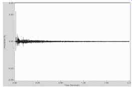
FIG. 15. The impulse response.
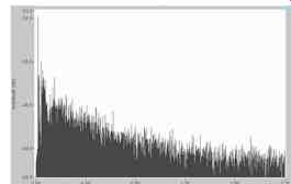
FIG. 16. The log-squared response.
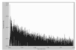
FIG. 17. The envelope-time curve (ETC).
3.5.4 Time Window Length
The time domain response can be divided to identify the portion that can be attributed to the loudspeaker and that which can be attributed to the room. It must be emphasized that there is a rather gray and frequency-dependent line between the two, but for this discussion we will assume that we can clearly separate them. The direct field is the energy that arrives at the listener prior to any reflections from the room. The division is fairly distinct if neither the loudspeaker nor microphone is placed near any reflecting surfaces, which, by the way, is a good system design practice. At long wavelengths (low frequencies) the direct field may include the effects of boundaries near the loudspeaker and micro phone. As frequency increases, the sound from the loud speaker becomes less affected by boundary effects (due in part to increased directivity) and can be measured independently of them. Proper loudspeaker placement produces a time gap between the sound energy arrivals from the loudspeaker and the later arriving room response. We can use this time gap to aid in selecting a time window to separate the loudspeaker response from the room response and diagnosing system problems.
3.5.5 Acoustic Wavelengths
Sound travels in waves. The sound waves that we are interested in characterizing have a physical size. There will be a minimum time span required to observe the spectral response of a waveform. The minimum required length of time to view an acoustical event is determined by the longest wavelength (lowest frequency) present in the event. At the upper limits of human hearing, the wavelengths are only a few millimeters in length, but as frequency decreases the waves become increasingly larger. At the lowest frequencies that humans hear, the wavelengths are many meters long, and can actually be larger than the listening (or measurement) space. This makes it difficult to measure low frequencies from a loudspeaker independently of the listening space, since low frequencies radiated from a loudspeaker interact (couple) with the surfaces around them. In an ideally positioned loudspeaker, the first energy arrival from the loudspeaker at mid- and high frequencies has already dissipated prior to the arrival of reflections and can therefore often be measured independently of them. The human hearing system tends to fuse the direct sound from the loudspeaker with the early reflections from nearby surfaces with regard to level (loudness) and frequency (tone). It is usually useful to consider them as separate events, especially since the time offset between the direct sound and first reflections will be unique for each listening position. This precludes any type of frequency domain correction (i.e., equalization) of the room/loudspeaker response other than at frequencies where coupling occurs due to close proximity to nearby surfaces. While it is possible to compensate to some extent for room reflections at a point in space (acoustic echo cancellers used for conference systems), this correction cannot be extended to include an area. This inability to compensate for the reflected energy at mid/high frequencies suggests that their effects be removed from the loudspeaker's direct field response prior to meaningful equalization work by use of an appropriate time window.
3.5.6 Microphone Placement
A microphone is needed to acquire the sound radiated into the space from the loudspeaker at a discrete position. Proper microphone placement is determined by the type of test being performed. If one were interested in measuring the decay time of the room, it is usually best to place the microphone well beyond critical distance.
This allows the build-up of the reverberant field to be observed as well as providing good resolution of the decaying tail. Critical distance is the distance from the loudspeaker at which the direct field level and reverberant field level are equal. It is described further in Section 3.5.7. If it's the loudspeaker's response that needs to be measured, then a microphone placement inside of critical distance will provide better data on some types of analyzers, since the direct sound field is stronger relative to the later energy returning from the room. If the microphone is placed too close to the loudspeaker, the measured sound levels will be accurate for that position, but may not accurately extrapolate to greater distances with the inverse-square law. As the sound travels farther, the response at a remote listening position may bear little resemblance to the response at the near field microphone position. For this reason, it is usually desirable to place the microphone in the far free field of the loudspeaker-not too close and not too far away. The approximate extent of the near field can be determined by considering that the path length difference from the measurement position (assumed axial) and the edge of the sound radiator should be less than 1/4 wavelength at the frequency of interest. This condition is easily met for a small loudspeaker that is radiating low frequencies.
Such devices closely approximate an ideal point source.
As the frequency increases the condition becomes more difficult to satisfy, especially if the size of the radiator also increases. Large radiators (or groups of radiators) emitting high frequencies can extend the near field to very long distances. Line arrays make use of this principle to overcome the inverse-square law. In practice, small bookshelf loudspeakers can be accurately measured at a few meters. About 10 m is a common measurement distance for moderate-sized, full-range loudspeakers in a large space. Even greater distances are required for large devices radiating high frequencies. A general guideline is to not put the mic closer than three times the loudspeaker's longest dimension.
3.5.7 Estimate the Critical Distance DC Critical distance is easy to estimate. A quick method with adequate accuracy requires a sound level meter and noise source. Ideally, the noise source should be band limited, as critical distance is frequency dependent. The 2 kHz octave band is a good place to start when measuring critical distance. Proceed as follows:
1. Energize the room with pink noise in the desired octave band from the sound source being measured. The level should be at least 25 dB higher than the background noise in the same octave band.
2. Using the sound level meter, take a reading near the loudspeaker (about 1 m) and on-axis. At this distance, the direct sound field will dominate the measurement.
3. Move away from the loudspeaker while observing the sound level meter. The sound level will fall off as you move farther away. If you are in a room with a reverberant sound field, at some distance the meter reading will quit dropping. You have now moved beyond critical distance. Measurements of the direct field beyond this point will be a challenge for some types of analysis. Move back toward the loudspeaker until the meter begins to rise again. You are now entering a good region to perform acoustic measurements on loudspeakers in this environment. The above process provides an estimate that is adequate for positioning a measurement microphone for loudspeaker testing. With a mic placement inside of critical distance, the direct field is a more dominant feature on the impulse response and a time window will be more effective in removing room reflections.
At this point it is interesting to wander around the room with the sound level meter and evaluate the uniformity of the reverberant field. Rooms that are reverberant by the classical definition will vary little in sound level beyond critical distance when energized with a continuous noise spectrum. Such spaces have low internal sound absorption relative to their volume.
3.5.8 Common Factors to All Measurement Systems
Let's assume that we wish to measure the impulse response of a loudspeaker/room combination. While it would not be practical to measure the response at every seat, it is good measurement practice to measure at as many seats as are required to prove the performance of the system. Once the impulse response is properly acquired, any number of post-processes can be performed on the data to extract information from it. Most modern measurement systems make use of digital sampling in acquiring the response of the system. The fundamentals and prerequisites are not unlike the techniques used to make any digital recording, where one must be concerned with the level of an event and its time length. Some setup is required and some fundamentals are as follows:
1. The sampling rate must be fast enough to capture the highest frequency component of interest. This requires at least two samples of the highest frequency component. If one wished to measure to 20 kHz, the required sample rate would need to be at least 40 kHz. Most measurement systems sample at 44.1 kHz or 48 kHz, more than sufficient for acoustic measurements.
2. The time length of the measurement must be long enough to allow the decaying energy curve to flatten out into the room noise floor. Care must be taken to not cut off the decaying energy, as this will result in artifacts in the data, like a scratch on a phonograph record. If the sampling rate is 44.1 kHz, then 44,100 samples must be collected for each second of room decay. A 3-second room would therefore require 44.1 × 1000 × 3 or 128,000 samples. A hand clap test is a good way to estimate the decay time of the room and therefore the required number of samples to fully capture it. The time span of the measurement also determines the lowest frequency that can be resolved from the measured data, which is approximately the inverse of the measurement length. The sampling rate can be reduced to increase the sampling time to yield better low-frequency information. The trade-off is a reduction in the highest frequency that can be measured, since the condition outlined in step one may have been violated.
3. The measurement must have a sufficient signal-to noise ratio to allow the decaying tail to be fully observed. This often requires that the measurement be repeated a number of times and the results averaged. Using a dual-channel FFT or MLS, the improvement in SNR will be 3 dB for each doubling of the number of averages. Ten averages is a good place to start, and this number can be increased or decreased depending on the environment. The level of the test stimulus is also important. Higher levels produce improved SNR, but can also stress the loudspeaker.
4. Perform the test and observe the data. It should fill the screen from top left to bottom right and be fully decayed prior to reaching the right side of the screen. It should also be repeatable. Run the test several times to check for consistency. Background noise can dramatically affect the repeatability of the measurement and the validity of the data.
Once the impulse response is acquired, it can be further analyzed for spectral content, intelligibility information, decay time, etc. These are referred to as metrics, and some require some knowledge on the part of the measurer in properly placing markers (called cursors) to identify the parameters required to perform the calculations. Let us look at how the response of the loudspeaker might be extracted from the data just gathered.
The time domain data displays what would have resulted if an impulse were fed through the system.
Don't try to correlate what you see on the analyzer with what you heard during the test. Most measurement systems display an impulse response that is calculated from a knowledge of the input and output signal to the system, and there is no resemblance between what you hear when the test is run and what you are seeing on the screen, FIG. 18.
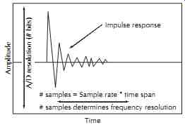
FIG. 18. Many analyzers acquire the room response by digital sampling.
Amplitude Time
# samples = Sample rate * time span
# samples determines frequency resolution A/D resolution (# bits) Impulse response 1»45
We can usually assume that the first energy arrival is from the loudspeaker itself, since any reflection would have to arrive later than the first wave front since it had to travel farther. Pre-arrivals can be caused by the acoustic wave propagating through a solid object, such as a ceiling or floor and reradiating near the microphone.
Such arrivals are very rare and usually quite low in level.
In some cases a reflection may actually be louder than the direct arrival. This could be due to loudspeaker design or its placement relative to the mic location. It's up to the measurer to determine if this is normal for a given loudspeaker position/seating position. All loud speakers will have some internal and external reflections that will arrive just after the first wave front. These are actually a part of the loudspeaker's response and can't be separated from the first wave front with a time window due to their close proximity without extreme compromises in frequency resolution. Such reflections are at least partially responsible for the characteristic sound of a loudspeaker. Studio monitor designers and studio control room designers go to great lengths to reduce the level of such reflections, yielding more accurate sound reproduction. Good system design practice is to place loudspeakers as far as possible from boundaries (at least at mid- and high frequencies). This will produce an initial time gap between the loudspeaker's response and the first reflections from the room. This gap is a good initial dividing point between the loudspeaker's response and the room's response, with the energy to the left of the dividing cursor being the response of the loud speaker and the energy to the right the response of the room. The placement of this divider can form a time window by having the analyzer ignore everything later in time than the cursor setting. The time window size also determines the frequency resolution of the post processed data. In the frequency domain, improved resolution means a smaller number. For instance, 10 Hz resolution is better than 40 Hz resolution. Since time and frequency have an inverse relationship, the time window length required to observe 10 Hz will be much longer than the time window length required to resolve 40 Hz.
The resolution can be estimated by f =1/T, where T is the length of the time window in seconds. Since a frequency magnitude plot is made up of a number of data points connected by a line, another way to view the frequency resolution is that it is the number of Hz between the data points in a frequency domain display.
The method of determination of the time window length varies with different analyzers. Some allow a cursor to be placed anywhere on the data record, and the placement determines the frequency resolution of the spectrum determined by the window length. Others require that the measurer select the number of samples to be used to form the time window, which in turn deter mines the frequency resolution of the time window. The window can then be positioned at different places on the time domain plot to observe the spectral content of the energy within the window, FIGs. 19, 20, and 21.
For instance, a 1 second total time (44,100 samples) could be divided into about twenty two time windows of 2048 samples each (about 45 ms). Each window would allow the observation of the spectral content down to ( ) × 1000 or 22 Hz. The windows can be overlapped and moved around to allow more precise selection of the time span to be observed. Displaying a number of these time windows in succession, each separated by a time offset, can form a 3D plot known as a waterfall.
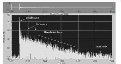
FIG. 19. A room response showing the various sound fields that can exist
in an enclosed space.
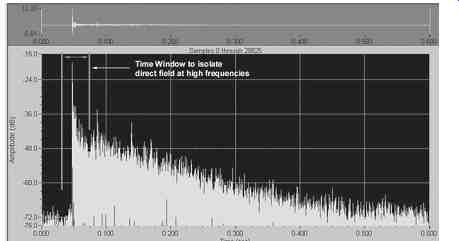
FIG. 20. A time window can be used to isolate the loudspeaker's response
from the room reflections.
3.5.9 Data Windows
There are some conditions that must be observed when placing cursors to define the time window. Ideally, we would like to place the cursor at a point on the time record where the energy is zero. A cursor placement that cuts off an energy arrival will produce a sharp rise or fall time that produces artifacts in the resultant calculated spectral response. Discontinuities in the time domain have broad spectral content in the frequency domain. A good example is a scratch on a phonograph record. The discontinuity formed by the scratch manifests itself as a broadband click during playback. If an otherwise smooth wheel has a discontinuity at one point, it would thump annoyingly when it was rolled on a smooth surface. Our measurement systems treat the data within the selected window as a continuously repeating event. The end of the event must line up with the beginning or a discontinuity occurs resulting in the generation of high-frequency artifacts called spectral leakage. In the same manner that a physical discontinuity in a phonograph record or wheel can be corrected by polishing, a discontinuity in a sampled time measurement can be remedied by tapering the energy at the beginning and end of the window to zero using a mathematical function. A number of data window shapes are available for performing the smoothing.
These include the Hann, Hamming, Blackman Harris, and others. In the same way that a physical polishing process removes some good material from what is being rubbed, data windows remove some good data in the process of smoothing the discontinuity. Each window has a particular shape that leaves the data largely untouched at the center of the window but tapers it to varying degrees toward the edges. Half windows only smooth the data at the right edge of the time record while full windows taper both (start and stop) edges.
Since all windows have side effects, there is no clear preference as to which one should be used. The Hann window provides a good compromise between time record truncation and data preservation. FIGs. 22 and 46-23 show how a data window might be used to reduce spectral leakage.
3.5.10 A Methodical Approach
Since there are an innumerable number of tests that can be performed on a system, it makes sense to establish a methodical and logical process for the measurement session. One such scenario may be as follows:
1. Determine the reason for and scope of the measurement session. What are you looking for? Can you hear it? Is it repeatable? Why do you need this information?
2. Determine what you are going to measure. Are you looking at the room or at the sound system? If it is the room, possibly the only meaningful measurements will be the overall decay time and the noise floor. If you are looking at the sound system, decide if you need to switch off or disconnect some loudspeakers. This may be essential to determine whether the individual components are working properly, or that an anomaly is the result of interaction between several components. "Divide and conquer" is the axiom.
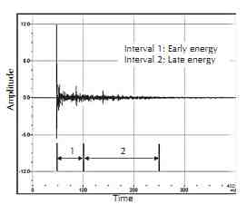
FIG. 21. Increasing the length of the time window increases the frequency
resolution, but lets more of the room into the measurement.
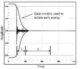
FIG. 22. The impulse response showing both early and late energy arrivals.
3. Select the microphone position. I usually begin by looking at the on-axis response of the loudspeaker as measured from inside of critical distance. If multiple loudspeakers are on, turn all of them off but one prior to measuring. The microphone should be placed in the far free field of the loudspeaker as previously described. When measuring a loud speaker's response, care should be taken to eliminate the effects of early reflections on the measured data, as these will generate acoustic comb filters that can mask the true response of the loudspeaker.
In most cases the predominant offending surface will be the floor or other boundaries near the microphone and loudspeaker. These reflections can be reduced or eliminated by using a ground plane microphone placement, a tall microphone stand (when the loudspeaker is overhead), or some strategically placed absorption. I prefer the tall micro phone stand for measuring installed systems with seating present since it works most anywhere, regardless of the seating type. The idea is to intercept the sound on its way to a listener position, but before it can interact with the physical boundaries around that position. These will always be unique to that particular seat, so it is better to look at the free field response, as it is the common denominator to many listener seats.
4. Begin with the big picture. Measure an impulse response of the complete decay of the space. This yields an idea of the overall properties of the room/system and provides a good point of reference for zooming in to smaller time windows. Save this information for documentation purposes, as later you may wish to reopen the file for further processing.
5. Reduce the size of the time window to eliminate room reflections. Remember that you are trading off frequency resolution when truncating the time record, FIG. 24. Be certain to maintain sufficient resolution to allow adequate low-frequency detail.
In some cases, it may be impossible to maintain a sufficiently long window to view low frequencies and at the same time eliminate the effects of reflections at higher frequencies, FIG. 25. In such cases, the investigator may wish to use a short window for looking at the high-frequency direct field, but a longer window for evaluating the woofer. Windows appropriate for each part of the spectrum can be used. Some measurement systems provide variable time windows, which allow low frequencies to be viewed in great detail (long time window) while still providing a semi-anechoic view (short time window) at high frequencies. There is evidence to support that this is how humans process sound information, making this method particularly interesting, FIG. 26.
6. Are other microphone positions necessary to characterize this loudspeaker? The off-axis response of some loudspeakers is very similar to the on-axis response, reducing the need to measure at many angles. Other loudspeakers have very erratic responses, and a measurement at any one point around the loudspeaker may bear little resemblance to the response at other positions. This is a design issue, but one that must be considered by the measurer.
7. Once an accurate impulse response is measured, it can be post-processed to yield information on spectral content, speech intelligibility, and music clarity. There are a number of metrics that can provide this information. These are interpretations of the measured data and generally correlate with subjective perception of the sound at that seat.
8. An often overlooked method of evaluating the impulse response is the use of convolution to encode it onto anechoic program material. An excellent freeware convolver called GratisVolver is available from www.catt.se. Listening to the IR can often reveal subtleties missed by the various metrics, as well as provide clues as to what postprocess must be used to observe the event of interest.
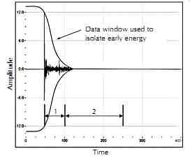
FIG. 23. A data window is used to remove the effects of the later arrivals.
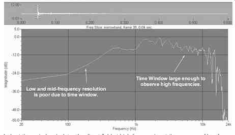
FIG. 24. A short time window isolates the direct field at high frequencies
at the expense of low-frequency resolution.
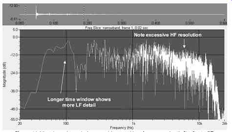
FIG. 25. A long time window provides good low-frequency detail.
3.6 Human Perception
Useful measurement systems can measure the impulse response of a loudspeaker/room combination with great detail. Information regarding speech intelligibility and music clarity can be derived from the impulse response.
In nearly all cases, this involves postprocessing the impulse response using one of several clarity measure metrics.
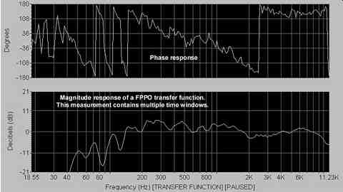
FIG. 26. The time window increases with length as frequency decreases.
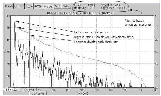
FIG. 27. The ETC can be processed to yield an intelligibility score, TEF25.
3.6.1 Percentage Articulation Loss of Consonants- (%Alcons)
For speech, one such metric is the percentage articulation loss of consonants, or %Alcons. Though not in widespread use today, a look at it can provide insight into the requirements for good speech intelligibility. A %Alcons measurement begins with an impulse response, which is usually displayed as a log-squared response or ETC. Since the calculation essentially examines the ratio between early energy, late energy, and noise, the measurer must place cursors on the display to define these parameters. These cursors may be placed automatically by the measurement program. The result is weighted with regard to decay time, so this too must be defined by the measurer. Analyzers such as the TEF25 and EASERA include best guess default placements based on the research of Peutz, Davis, and others, FIG. 27.
These placements were determined by correlating measured data with live listener scores in various acoustic environments, and represent a defined and orderly approach to achieving meaningful results that correlate with the perception of live listeners. The measurer is free to choose alternate cursor placements, but great care must be taken to be consistent. Also, alternate cursor placements make it difficult if not impossible to compare your results with those obtained by other measurers. In the default %Alcons placement, the early energy (direct sound field) includes the first major sound arrival and any energy arrivals within the next 7-10 ms. This forms a tight time span for the direct sound. Energy beyond this span is considered late energy and an impairment to communication. As one might guess, a later cursor placement yields better intelligibility scores, since more of the room response is being considered beneficial to intelligibility. As such, the default placement yields a worst-case scenario. The default placement considers the effects of the early-decay time (EDT) rather than the classical T30 since short EDTs can yield good intelligibility, even in rooms with a long T30. Again, the measurer is free to select an alternative cursor placement for determining the decay time used in the calculation, with the same caveats as placing the early-to-late dividing cursor. The
%Alcons score is displayed instantly upon cursor placement and updates as the cursors are moved.
3.6.2 Speech Transmission Index-(STI) The STI can be calculated from the measured impulse response with a routine outlined by Schroeder and detailed by Becker in the reference. The STI is probably the most widely used contemporary measure of intelligibility. It is supported by virtually all measurement plat forms, and some handheld analyzers are available for quick checks. In short, it is a number ranging from 0 to 1, with fair intelligibility centered at 0.5 on the scale.
For more details on the Speech Transmission Index, see the section on speech intelligibility in this text.
3.7 Polarity
Good sound system installation practice dictates maintaining proper signal polarity from system input to system output. An audio signal waveform always swings above and below some reference point. In acoustics, this reference point is the ambient atmospheric pressure. In an electronic device, the reference is the 0 VA reference of the power supply (often called signal ground) in push-pull circuits or a fixed dc offset in class A circuits.
Let's look at the acoustic situation first. An increase in the air pressure caused by a sound wave will produce an inward deflection of the diaphragm of a pressure micro phone (the most common type) regardless of the micro phone's orientation toward the source. This inward deflection should cause a positive-going voltage swing at the output of the microphone on pin 2 relative to pin 3, as well as at the output of each piece of equipment that the signal passes through. Ultimately the electrical signal will be applied to a loudspeaker, which should deflect outward (toward an axial listener) on the positive-going signal, producing an increase in the ambient atmospheric pressure. Think of the microphone diaphragm and loudspeaker diaphragm moving in tandem and you will have the picture. Since most sound reinforcement equipment uses bipolar power supplies (allowing the audio signal to swing positive and negative about a zero reference point), it is possible for signals to become inverted in polarity (flipped over). This causes a device to output a negative-going voltage when it is fed a positive-going voltage. If the loudspeaker is reverse-polarity from the microphone, an increase in sound pressure at the microphone (compression) will cause a decrease in pressure in front of the loudspeaker (rarefaction). Under some conditions, this can be extremely audible and destructive to sound quality. In other scenarios it can be irrelevant, but it is always good to check.
System installers should always check for proper polarity when installing the sound system. There are a number of methods, some simple and some complex.
Let's deal with them in order of complexity, starting with the simplest and least-costly method.
3.7.1 The Battery Test
Low-frequency loudspeakers can be tested using a standard 9V battery. The battery has a positive and negative terminal, and the spacing between the terminals is just about right to fit across the terminals of most woofers.
The loudspeaker cone will move outward when the battery is placed across the loudspeaker terminals with the battery positive connected to the loudspeaker positive.
While this is one of the most accurate methods for testing polarity, it doesn't work for most electronic devices or high-frequency drivers. Even so, it's probably the least-costly and most accurate way to test a woofer.
3.7.2 Polarity Testers
There are a number of commercially available polarity test sets in the audio marketplace. The set includes a sending device that outputs a test pulse, FIG. 28, through a small loudspeaker (for testing microphones) or an XLR connector (for testing electronic devices) and a receiving device that collects the signal via an internal microphone (loudspeaker testing) or XLR input jack. A green light indicates correct polarity and a red light indicates reverse polarity. The receive unit should be placed at the system output (in front of the loudspeaker) while the send unit is systematically moved from device to device toward the system input. A polarity reversal will manifest itself by a red light on the receive unit.
3.7.3 Impulse Response Tests
The impulse response is perhaps the most fundamental of audio and acoustic measurements. The polarity of a loudspeaker or electronic device can be determined from observing its impulse response, FIGs. 29 and 46-30. This is one of the few ways to test flown loud speakers from a remote position. It is best to test the polarity of components of multiway loudspeakers individually, since all of the individual components may not be polarized the same. Filters in the signal path (i.e., active crossover network) make the results more difficult to interpret, so it may be necessary to carefully test a system component (i.e., woofer) full-range for definitive results. Be sure to return the crossover to its proper setting before continuing.
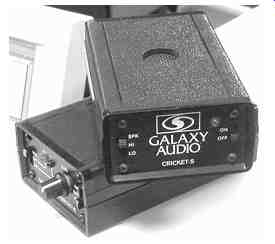
FIG. 28. A popular polarity test set.
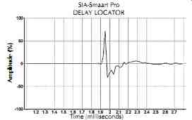
FIG. 29. The impulse response of a transducer with correct polarity.
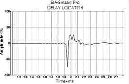
FIG. 30. The impulse response of a reverse-polarity transducer.
4 Conclusion
The test and measurement of the sound reinforcement system are a vital part of the installation and diagnostic processes. The FFT and the analyzers that use it have revolutionized the measurement process, allowing sound practitioners to pick apart the system response and look at the response of the loudspeaker, roo, or both. Powerful analyzers that were once beyond the reach of most technicians are readily available and affordable, and cost can no longer be used as an excuse for not measuring the system. The greatest investment by far is the time required to grasp the fundamentals of acoustics to allow interpretation of the data. Some of this information is general, and some of it is specific to certain measurement systems.
The acquisition of a measurement system is the first step in ascending the capability and credibility ladder.
The next steps include acquiring proper instruction on its use by self-study or short course. The final and most important steps are the countless hours in the field required to correlate measured data with the hearing process. As proficiency in this area increases, the speed of execution, validity, and relevance of the measurements will increase also. While we can all learn how to make the measurements in a relatively short time span, the rest of our careers will be spent learning how to interpret what we are measuring.