Build an Engine Analyzer
If you are anything like most hobbyists, you hate to pay someone else to do something you can do yourself. That's the way it is with many experimenters and their automobiles. They are self-professed experts, yet have no way of taking on the complexities of the common Kettering automobile ignition system.
For this project, get your hands on an automotive timing light. It has a bright flash and operates from the car battery system. Hook it up to your car.
The instructions say to hook the red and black wires on the light to the positive and negative terminals of the car battery and then clamp the induction pickup around the number one spark plug wire. Elementary, so far. With the engine running, and being careful to watch that those dangling wires don't drop into the spinning fan blades, gently squeeze the trigger on the gun and watch the light spring to life.
One hobbyist tried this and since he had fiddled around some with automotive problems and knew that the timing marks are found on the side of the front pulley he figured that all that had to be done was to rub some chalk into those marks. Then you can see them easily, and, with the timing light aimed at the spinning pulley,, press the trigger and watch the strobing action as the number one cylinder fires the timing light.
However, he did overlook a few small details. The vacuum advance line to the distributor must be pulled and plugged according to the manufacturer's directions. Also, "Timing must be adjusted with the engine running at manufacturer's specified rpm. If necessary, use a tachometer to set idle rpm." Not having a tachometer, the first thought that went through this hobbyist's mind was to run out and buy one. Somehow that didn't settle too well with him. He needed to figure how many revolutions per minute his little Pinto engine was turning over however, and with a fair degree of accuracy.
We've all seen the modern, automotive electronics shops, with their big engine analyzer scopes all nicely calibrated, but who among us is going to rush out and buy one of those! What this hobbyist did have was a pretty fair B and K model 1461, 10 MHz, triggered oscilloscope, with 18 calibrated sweep ranges.
The problem was interesting. He began by thinking in terms of how the combustion engine works. It takes a fuel/air mixture into the cylinder on a downstroke, compresses it on the up-stoke, where it begins burning the mixture by sparking the plug somewhere before top dead center. The resultant explosion gives the power downstroke. Finally, the cylinder on the last upstroke exhausts the by-products of burning. The problem is to fire the plug at just the correct time on the first upstroke before top dead center and do this timing with the engine running at a specified number of revolutions per minute. The timing light flashing on the timing marks will show the answer to the first problem, but that rpm problem must still be figured out.
Remember, that cylinder fires only once for every two engine revolutions.
What we must do is get a good, stationary display of all cylinders firing on the scope, so we can measure the duration of all cylinder firings in time.
With an externally triggered scope, this is a cinch. Take a clip lead and loosely couple it around the number one spark plug wire. Just use an ordinary clip lead with an alligator clip on one end. Clipping this around the plug wire gives plenty of induced pulses to easily trigger the scope. Switching to external trigger, the scope will now make one sweep, from left to right across the tube, for every firing of that number one cylinder. Then, by coupling the vertical input of the scope to the high tension lead coming out of the center of the distributor in the same manner, your display will show the firings of all cylinders in exactly the sequence they actually are firing. In the case of the Pinto, it will be, first, number one cylinder, followed by three, four, and finally, number two. It's a simple matter to immediately see if all plugs are firing, and also to see the relative amplitude of the spark voltage to each cylinder. The vertical gain control, along with the vertical positioning control, can be used to bring the voltage peaks of all firings onto the scope face. Just remember, we are only looking at induced voltage through the insulation of the spark plug wire. We have not connected our scope directly to any bare wire, as the plug wires can carry well over 10,000 volts of AC. In some cases, it may help to put a 2200 ohm resistor and . 05 capacitor across the input of your scope to dampen out much of the high frequency information we are not interested in. Some experimentation is called for with the exact values. Nothing is very critical in this department. Time in seconds is the reciprocal of frequency in Hertz, and frequency in Hertz is the reciprocal of time in seconds.
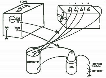
Fig. 11-1. Scope connections.
Remember, we want to measure engine revolutions in time - specifically, revolutions per minute. Because, as stated above, frequency in Hertz is the reciprocal of time in seconds. All we must do is measure, with the scope, the time for all cylinders to fire, take the reciprocal of this time in seconds to get frequency in Hertz, and then multiply by 120, thereby getting revolutions per minute. (Remember, that cylinder fires once every other revolution; therefore we must multiply by 120 rather than 60.) If we look at a calibrated sweep oscilloscope, we see that sweep time is usually measured in milliseconds or microseconds per division on the graticule over the face of the tube. All we must do is count the number of divisions, generally centimeters, multiply by the indicated number of milliseconds or microseconds per division of the sweep time scale of the scope, and take the reciprocal to find frequency. At this point, a small calculator is an immense help, unless you like to do long division with a pencil.
As an example, suppose we have connected our scope as shown in Fig. 11-1, and we are driving a four-banger. Our sweep time is set for 5 milliseconds percentimeter. The time between firings is 6.6 centimeters.
Multiplying this by the sweep time of 5 milliseconds percentimeter, we find that time between firings is 33 milliseconds, or 132 milliseconds for four cylinders. Taking the reciprocal of 132 milliseconds and multiplying by 120 reveals engine revolutions to be 909 revolutions per minute.
Although the scope could have been set up for a display of all four cylinder firings, a little more accuracy is possible by using an expanded sweep and measuring the time for one cylinder firing, rather than by multiplying by the total number of cylinders. There probably isn't much difference, so it will boil down to what each individual feels most comfortable with.
To set the curb idle speed of your car, it is always best to refer to the manufacturer's specs, either in the owner's manual or in a local library, in a good automotive manual. Generally, it's a matter of adjusting the correct screw on the carburetor. Curb idle speeds will vary, and the specs may call out different rpm for such cases as cars equipped with or without air conditioning, etc. Once the idle speed has been properly set, the timing can be adjusted with the light. This involved loosening the lock nut under the distributor and gently turning the distributor, while watching the timing marks on the front pulley in the strobing flash of the timing light. Timing will also increase or decrease the engine rpm, so you may find yourself going back and tweaking the curb idle adjust again.
A word of caution is called for here. Adjustment of engine timing and curb idle speed will affect the emissions of your car. Go slowly the first time, consult your manuals and set your car up by the book. Don't forget to reconnect the vacuum line back onto the distributor when you are finished.
At today's prices for automotive analysis and tune-up, it won't take long before this simple equipment will pay for itself.
Your ' Scope Can Be Improved
The oscilloscope is one of the most versatile instruments in the hob byist's workshop and it would probably take an entire book just to list its many uses. Quite a few of the lower priced instruments, however, are handicapped by the fact that, though they can faithfully display the shape of the waveform under examination, they cannot be used to accurately measure the amplitude or the frequency of the signal. This is true not because there is anything wrong with the instruments themselves, but simply be cause most of them do not have build-in calibration circuits, or they have only very rudimentary ones.
Amplitude calibration is normally carried out by applying a signal or voltage of known amplitude to the vertical input of the oscilloscope and adjusting the vertical gain control until the displayed signal spans a given number of divisions on the reticle. You then have a known calibration value in volts per division (V/div.), and the amplitude of any unknown signal or voltage can be read directly from the screen.
The scope's vertical input attenuator can be used to accurately measure higher voltages. For example, if you calibrate the scope to read 1 V/div., then, by simply turning the attenuator switch to the X10 position, it will be calibrated at 10 V/div. You can go the other way, too. For example, start out with the attenuator in the X10 position and calibrate the scope to display 1 V/div. Then turn the attenuator back to Xl, and the scope will be calibrated at 0.1 V/div. (i.e., 100 mV/div.). Frequency measurements are handled in a similar fashion, but by using the horizontal sweep frequency and/or gain controls to calibrate the horizontal axis such that the signal of known frequency is displayed with a given number of cycles per division. The frequency of an unknown signal can then be measured by noting the number of cycles per division it occupies on the screen.
Some oscilloscopes have a built-in calibration signal, but often consist of nothing more than an extra winding on the power transformer to supply 1 volt peak-to-peak at 60 Hz. Consequently, any line voltage changes would cause the amplitude of the calibration signal to change by the same percentage, which is entirely unacceptable for accurate measurements. The frequency is that of the line itself and, consequently, extremely accurate.
However, 60 Hz is such a low frequency compared to the signals normally being measured in the audio range that the measurements which are possible in theory are not possible in practice because of the great percentage difference (that is, the ratio) between the reference signal and the unknown signal.
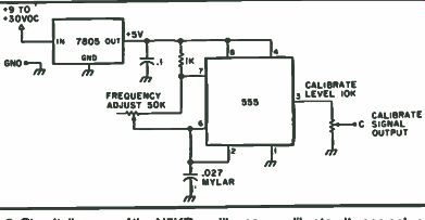
Fig. 11-2. Circuit diagram of the N5KR oscilloscope calibrator. It uses only
seven components, all of which are readily available.
The solution to all these problems is the circuit shown in Fig. 11-2, which generates a stable wave calibration signal and costs less than $3 to build. The component values shown have been selected to provide a sym metrical 1-volt p-p signal at 1000 Hz when the two trimpots are calibrated.
The 555 timer generates the signal at a stable frequency, while the 7805 regulator ensures a fixed amplitude. The entire circuit contains only seven components, which are mounted on a small PC board as shown in Fig. 11-3.
The 1v p-p signal enables fast and simple calibration of the scope in the vertical (amplitude) axis, and the 1000 Hz frequency is a nice round reference frequency for analysis of most audio signals. The circuit board is small enough to mount inside of the oscilloscope itself, with the few milliamps of power required being supplied from the scope's existing power supply.
Construction. The circuit is simple enough to build on perfboard, and parts layout is not critical. It can be built on a small PC board, the layout for which is shown in Fig. 11-4. Parts placement, as viewed from the component side, is given in Fig. 11-5.
Component tolerances of 20 percent are satisfactory, since the two trimpots are used to make the final amplitude and frequency adjustments. In fact; the . 027 ¡ if capacitor can be substituted with any value from . 02 to 0.047, if you don't have a 0.027. But it would be better to go lower in value rather than higher, if you have a choice. The important thing is that this capacitor be of mylar or other temperature-stable type. The PC layout shown in Fig. 11-4 has two different solder pads (one on an extension) on the ground side of this capacitor to accommodate whatever capacitor you select, since its physical size may be different from the one used here. There are also a couple of extra solder pads for making an external ground connection, if desired.
The 7805 regulator may be substituted for an LM340T-5, which is the same device. On rare occasions, these regulators have been known to go into self-oscillation. Should you encounter this problem, replacing the 0.1 uF disc capacitor with a le tantalum capacitor should clear it up.
Mounting and Power Connections. The circuit is so small that it can be mounted almost anywhere in the scope. In fact, you can trim the PC board down a lot smaller than the one shown in Fig. 11-3, which has a lot of blank space around the edges. You should, however, make it a point to mount it as far as possible from major heat sources so that the calibrator's frequency stability won't be impaired.
The input voltage can be anywhere from +9 to +30 volts DC, and you won't have any trouble finding a supply voltage somewhere in this range in a solid state oscilloscope. If your scope is tube type, you might still find a
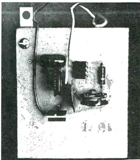
Fig. 11-3. Photograph of the finished board ready for installations in the
scope.
The trimpot at the lower right sets the frequency, while the one toward the left sets the amplitude of the calibrate signal.
voltage of the proper value, but if not, you can obtain it from a higher voltage through an appropriate voltage divider. The supply voltage doesn't have to be regulated, but, on the other hand, you want to avoid one that fluctuates widely. The negative (ground) connection can be made through the mounting bracket, if desired.
If your scope has an existing jack on the front panel for a calibrate signal, just disconnect the wire from the existing calibrate signal and run a new wire from the jack to the calibrate signal output (C) on the circuit board. If you don't already have a jack or if you want to retain your existing calibrate signal, you will need to mount a small pin jack on the front panel for this connection.
Calibration. In order for the calibrator to be of any use, it must itself be calibrated in an accurate manner, and the circuit has been designed for simplicity in that respect. First, set the two trimpots to mid-scale. Now, with power applied to the calibrator circuit, use a VTVM or other accurate ...
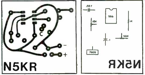
Fig. 11-4. PC layout, foil- side view.
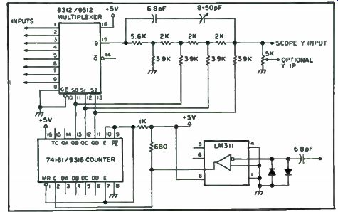
Fig. 11-5. Parts placement, component-side view.
... voltmeter to measure the calibrate signal at C. Set the voltmeter to read "DC volts," and adjust the 10k pot until the meter reads exactly one-half volt (0.5 V). What you have done here is used the DC voltmeter to measure the average output voltage, and, since the signal is switching back and forth between 0 volts and 1 volt, the average value you read on the meter is 0.5 volts. This is true only for a symmetrical square wave, of course, and the component values in this circuit have been chosen such that any error in symmetry is less than 1 percent at 1000 Hz. You also have to be assured that the negative (low) half cycle of the signal is actually at zero volts, which it is, for all practical purposes, when the 555 is operated at the 5v input voltage supplied by the 7805 regulator.
The easiest way to set the frequency is to measure the calibrate signal with a digital counter. If you don't have access to one, an accurate audio signal generator can be used, with the calibrate signal frequency being adjusted to match the known signal while they are being watched on the scope. In any case, the frequency of the calibrate signal is adjusted with the 50k pot.
If you prefer a frequency other than 1000 Hz, you can set the pot for a lower frequency without hurting anything. If you set the pot to a higher frequency, though, the symmetry of the waveform will be upset. To go to a higher frequency, you should lower the value of the 0.027 capacitor instead, using the formula: C = 28/F, where C is the value in microfarads of the new capacitor, and F is the desired signal frequency.
Summary. This is one of those satisfying projects that you can put together in an hour or so, at a cost of only $2 or $3 and see the results immediately. It consists of only seven components, which are available from any retail or mail-order electronics dealer. It's a handy little device that will enhance the utility of lower cost oscilloscopes and you can sit back and enjoy using it for years to come.
Eight Trace Scope Adapter
Probably the most frustrating problem faced when designing digital circuitry is control of timing. After working out a design on paper, one usually breadboards the circuit to prove it out. In accordance with Murphy's well-known laws, there will be several logic errors which will then be apparent but very elusive. Depending upon the complexity of the design, the errors may be (but usually are not) easily located and corrected.
A number of tools are helpful in tracking down these problems-the logic probe and oscilloscope probably being the most helpful. A logic probe establishes the steady-state status of various points in the circuit, but tells nothing about pulse widths or repetition rates. The oscilloscope is used to visually illustrate these waveshapes, pulse widths and repetition rates.
What most scopes do not show is the time relationship between pulses at different locations in the circuit. Sometimes this relationship is crucial in searching out a problem that may be caused by glitches ( extremely short pulses caused by unexpected and unwanted time overlaps). Well-equipped laboratories use special multichannel logic scopes for this sort of work, but most of us are not equipped with the kilo-buck pocketbook required to manage this. Even a dual channel high speed scope requires a considerable investment.
While such a scope would be most welcome in any experimenter's laboratory, most of us must settle for a relatively inexpensive general purpose scope. Fortunately, it is neither difficult nor expensive to build an adapter to display multichannel logic signals. The adapter permits viewing up to eight channels of logic signals simultaneously, and thereby examination of the relative timing between them. Although analog waveshapes cannot be ...
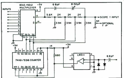
Fig. 11-6. Schematic.
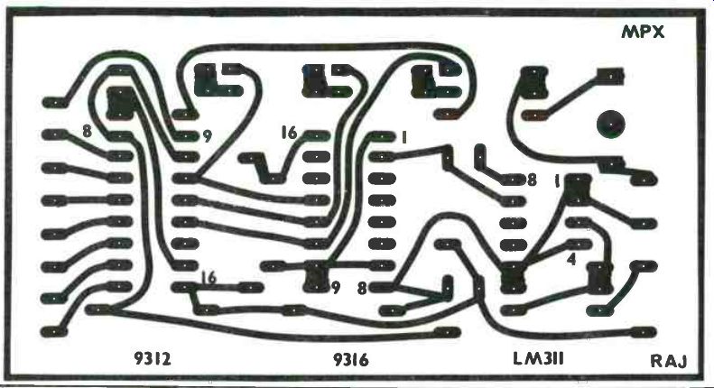
Fig. 11-7. PC board (full size).
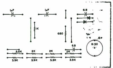
Fig. 11.8
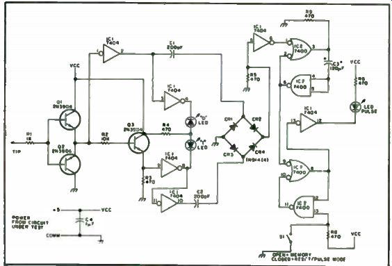
Fig. 11-9. Component layout.
... displayed (you can use your scope without the adapter for this function), it will show the low or high states, in precise time positions, of any signals present in TTL or DTL circuits.
Almost any general purpose scope should work with this adapter, but it is recommended that it be equipped with a triggered sweep. The viewing of simple repetitive signals without a triggered sweep can be frustrating enough, but attempting to lock onto one of eight channels being displayed may be virtually impossible. If you are using a scope without this feature, consider adding a new triggered sweep, even if you do not build this adapter.
Scope bandwidth is not critical unless you are working with really high speed stuff, and a 4 MHz bandwidth will let you examine almost all you need to see. You must have a way to externally trigger the scope sweep, and you will have to find the sweep signal or blanking pulse to permit changing the input channels during the retrace interval.
The circuit itself is very simple. A small capacitor couples the scope sweep circuit to a voltage comparator (you may find it necessary to adjust the size of the capacitor for reliable trace switching). The sweep retrace causes a negative excursion at pin 3 of the LM311, forcing its output to go high. Each time this occurs, a 16 stage counter advances one count. Three output bits of the counter are connected to an eight-to-one 9312 multiplexer, which selects each input in turn and outputs to pin 15. If most of your work is at the lower frequencies, use the low order 3 bits of the counter, instead of the 3 high order bits (Fig. 11-6). When using the 3 high order bits, you may use the adapter with a fuel channel scope operating in the alternate mode.
A ladder network commonly used for digital to analog conversion is used to position each channel on the screen. The resistors should be well matched (i.e., 1 percent), but satisfactory results have been experienced with 5 percent units. If your display is not evenly spaced vertically, try swapping resistors in this network for best spacing. The variable capacitor is used to compensate for the scope input capacitance, and should be adjusted for best waveshapes. The output potentiometer will not be required in most instances, and should not be used unless essential.
Note in Fig. 11-6 that a 74161 or 9316 synchronous counter is recom mended, rather than a 7493 or similar asynchronous type. It is unlikely that propagation delays in an asynchronous counter would result in viewable glitches on the scope in this application, but it is good design practice to always use a synchronous counter where the output states are decoded and fed back to the counter.
The adapter may be built on a small printed circuit board (Fig. 11-7) and installed inside your scope. However, it may be very conveniently enclosed in a small box which can be located near and powered from the digital project, and coupled to the scope via cables. You will need the usual vertical input cable and a sweep-out signal. Many scopes have an Ext jack for horizontal input, which is permanently connected to the input of the horizontal amplifier. When the sweep is running, this also happens to be the output of the sweep generator.
Should you experience difficulty in obtaining a stable trace, the sweep circuit may not be advancing the counter properly. Try a different spot in the sweep circuit first. You may find it necessary to invert the signal by using pin 2 of the LM311 (grounding pin 3) if the signal is reversed in polarity. The 74161 counts on a rising edge, and reverse polarity will cause the channel change to occur in mid-sweep, with obvious visible distortion. You may find experimenting with the size of the sweep input capacitor to be helpful, but be careful to avoid distorting the sweep. The scope will not be as bright as usual, as the trace is being timeshared among 8 signals. A slight adjustment of the brightness control compensates for this. The variable capacitor is adjusted for best waveform using a 10 kHz or higher digital pulse. A 74151 ...
Fig. 11-9. The Superprobe. * Note: C3 is two small 60 uF caps wired in parallel.
------------------
IC1 -SN7404 IC IC2 -SN7400 IC QI, Q3 -2N3904 transistor
Q2 2N3906 transistor CR1, 2, 3, 4 -1N914 diode R1 -1k 1/4 Watt resistor R2 -10k 1/4 Watt resistor R3-9 -470 Ohm 1/4 Watt resistors Cl, C2 -200 pF capacitor C3 -120 elf capacitor (2 small 60 MF inparallel)
C4 -. 1 1.4.F disc capacitor LED 1-3 -Any type/color LED desired
Table 11-1. Parts List

---------------------
... multiplexer is functionally identical, but not pin compatible, with the 9312 unit. The LM311 comes in either a mini-dip or TO-5 package. As the pin-outs are identical, either may be used with the circuit board shown (Fig. 11-8). Using your multitrace scope is a delightful experience: You see all of those signals at the same time, and can really tell what is going on. Re member that you must trigger the sweep from the slowest signal you are viewing. Otherwise, you will not be able to sync the slower signals. Also, be aware that the inputs are not protected in any way, and connection to potentials outside of the proper logic levels will destroy the multiplexer IC. Protective diodes may be added on the input lines to give marginal security, but care, plus a socket for the 9312, are probably adequate.
The small investment required to construct this unit will be quickly repaid the first time you use it to track down a problem.
Superprobe If the modern technician is going to be successful when working with digital logic, he must have means of looking inside the circuit. The most common way in the industry is with the use of an oscilloscope or logic analyzer. Both of these instruments are great, but the cost puts them out of reach for most experimenters.
The Superprobe ( Fig. 11-9) was designed to be an inexpensive piece of test gear which will provide the necessary insight into the digital circuit under test. This probe is not a toy, and will provide the user with almost as much information as a $3,000 oscilloscope, when dealing with TTL or DTL logic.
The probe has several desirable features, aside from the expected "1" and "0" indication. The first is a pulse stretcher, and pulse memory. Any time a high to low or low to high transition takes place, the pulse LED will flash. The flash will be visible even with very narrow pulses, since the probe will stretch the pulse width to a visible flash. If the probe is in the memory mode, the pulse LED will remain lit until reset by the operator, capturing any stray pulse. Another important feature is high impedance input. It will not load the circuit under test. The input is protected by the zener action of the input transistors, with current limited by R1, in the event the probe is touched to high voltage.
Yet another feature of this probe is that if the tip is touched to an open circuit, or to a chain of floating inputs, no light will light, thus identifying this condition immediately. The entire circuit uses only two inexpensive TTL ICs, three transistors, and can be built into a handy, hand-held probe. The parts list is found in Table 11-1.
The Audible Probe Is Safer to Use
This project is a piece of test gear that gives the output in audio. The unit does not have to fit totally in the hand since it's for bench work.
Therefore, creation of the sound (loudspeaker) won't be a problem.
You can now build a logic probe that works with CMOS, produces a high tone for a logic high, a low tone for a logic low and no sound for an open or floating string. In addition to this, the unit will detect narrow pulses and stretch them so the user is able to hear them.
The audio probe will detect high to low, or low to high pulses and will do anything any good probe will do, except its output is in sound. It works great!
Circuit Description. Transistors Q1 and Q2 form the input stage (Fig. 11-10). Under no signal or floating input condition, both transistors are biased on by the base resistors. In the ON state, the collector of Q1 is near ground and the collector of Q2 is near plus volts. It is stated as "near" because of the 3 volt zeners in the emitter of each transistor. The zeners will subtract their voltage from what is developed in the collector circuit. The purpose of the zeners is to provide a threshold level at which the transistor will key. For Q1 to turn on, the base must be greater than 3.5 volts, and for Q2 to turn off, its base must be higher than supply voltage minus 3.5 volts.
This choice of zener value is not critical. The choice for this project was made based on the fact that all of the cmos circuits are run from 12 volts.
With this value of zener, the probe rejects any signal not below 3.5 or above 9 volts. A functioning circuit will easily exceed these values, and if it won't, the circuit is bad. From this point on, think logic. We will call the collector of Q1 "A," and the collector of Q2 "B." If the probe tip is floating, A is low and B is high. li the tip is low, A is high and B is also high. If the tip is high, A is low and B is also low.
Three unique states-one for each condition. Now all that is necessary is to decode the states. Only the 1 and 0 states are decoded, since if the state is not a 1 and 0, it must be the open state and nothing happens during this state. If a high condition occurs, the 1 decoder triggers the pulse stretcher.
This pulse stretcher is a bit different in that it uses an OR gate. If pin 1 goes high, pin 3 also goes high, feeding back through C1 holding pin 2, and itself high for the time determined by the time constant of C1 and R5. When Cl/R5 time out, the output of pin 3 will drop low again if there is not a high still on pin one. The gate acts like a straight piece of wire except that it will stretch a short pulse. Any time the output of pin 3 is high, it will enable the high pitch oscillator, causing a high tone to be generated.
Fig. 11-10. Circuit description. LOW PULSE STRETCHER LOW TONE OSCILLATOR.
The 0 decode, pulse stretcher and oscillator work exactly the same as the circuit just described, except, of course, the tone generated is a low pitch. The two tones generated are mixed in the final section of IC3, with the inputs on pins 8 and 9, and the mixed audio on pin 10. The output at pin 10 is good for an earphone (used with a volume control) or a small speaker. You could even add a small audio amplifier if you work in a noisy environment. Of course, it could blast you out of the room. As mentioned, the unit will produce a high tone for a high and a low tone for a low. With a bit of practice, as with other types or probes, you can get a pretty good idea of what is going on by the sound. If it sounds like both tones are on, you have a square wave signal. If you have a high tone with a low tone ticking, you have a high with a low pulse, and so on. For a parts list for this project, see Table 11-2.
Mod for the Heath 10-102 Scope
The Heath 10-102 scope kit appears to be one of the "better buys for the money." The 30 mV vertical sensitivity, 80 nanosecond rise time, and 5 MHz frequency response seem to fill the bill. Actually, the vertical response is adequate for viewing 15 MHz or higher signals with sufficient trace height to be usable. Assembly is on four main circuit boards: vertical, horizontal, sweep and power supply. The finished unit is uncluttered, internal adjust ments are no problem and most components are easily serviced.
Critical power supply voltages are zener regulated, a fact which contri butes to the operational stability after warm-up. The power transformer, which is double shielded, and circuit board layout result in a trace like those drawn in textbooks.
The initial alignment and internal adjustments, although not difficult, must be performed as directed. An accurate VOM or VTVM is the only equipment needed. During this alignment, one wishes he had a screwdriver with a 10 to 1 drive. However, with a light touch, the desired results can be achieved.
Heath states that vertical drift during warm-up "for the first half hour or so" is to be expected. Experience with two of these units was as follows: From a cold start at 70°F, the trace was completely off the screen for the first 10 minutes. After 10 minutes, the trace appeared at the top of the CRT and drifted downward for 35 minutes, at which time it stabilized and no further drift was noted over several hours of operation. For someone who turns on the instrument and intends to use it all day, this may not appear as a problem. You may find juggling the vertical position control inconvenient, especially if your use is on an intermittent basis. The addition of four simple heat sinks produced two improvements:
• A usable trace on the screen in 3 to 4 minutes.
• A completely stable trace, without touching the position control, in 12 to 15 minutes.
Two heat sinks were made from aluminum and attached to the vertical output transistor heat sink tabs. The tops of these sinks, which were bent 90°, may be secured to the CRT shelf with standoff insulators or RTV
---------------
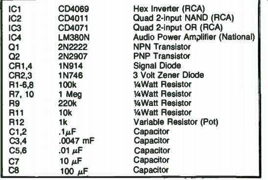
Table 11-2. Parts List.
IC1 CD4069 Hex Inverter ( RCA) IC2 CD4011 Quad 2-input NAND ( RCA) IC3 CD4071 Quad 2-input OR ( RCA) IC4 LM380N Audio Power Amplifier ( National)
Q1 2N2222 NPN Transistor
Q2 2N2907 PNP Transistor CR1,4 1N914 Signal Diode CR2,3 1N746 3 Volt Zener Diode R1-6,8 100k 1/4 Watt Resistor R7, 10 1 Meg 1/4 Watt Resistor R9 220k 1/4 Watt Resistor R11 10k 1/4 Watt Resistor R12 1k Variable Resistor (Pot)
C1,2 .1uF Capacitor
C3,4 .0047 mF Capacitor
C5,6 .01 ALF Capacitor C7 10 uF Capacitor C8 100 uF Capacitor
-----------------------------
... cement. Two additional heat sinks, 1" by 1", were attached to the driver transistors with a small wrap-around wire.
Heath incorporates a 1 volt peak to peak calibrating signal at a front panel jack. A square wave calibrating signal and incorporated circuit are used. The calibrator provides a clipped sine wave signal of 0.1v, 1v and 10v.
Three pin jacks were added next to the vertical input ground jack, to bring these signals to the front panel from the circuit which was mounted on the cover of the power supply transformer using existing screws.
--
Next: RF Test Equipment