A perspective view of the subject of electrical noise and its origins
by Professor D.A.BELL, F.Inst. P., F.I.E.E.
Noise, which in electronics and communication is the traditional name for random fluctuations or disturbances, is of fundamental importance because it sets an absolute limit to the performance of systems of communication, including measuring devices and transducers. In papers published in 1948, Shannon' established the foundations of modern communication theory and stated the fundamental limitations as follows:
"If the channel is noisy it is not in general possible to reconstruct the original message or the transmitted signal with certainty by any operation on the received signal E." Note that he emphasized with certainty:
an enormous amount of work has been expended on error-correcting codes which allow the reconstruction of the original message to a high degree of probability (low probability of error) but signal-to-noise ratio remains a fundamental parameter of all systems. The two forms of noise which are fundamental and simply defined are thermal and shot noise, though the development of solid-state devices has brought forward avalanche noise, the peculiarities of noise in Gunn effect devices and the still unexplained VI noise.
THERMAL NOISE
Since all electrical conduction depends on the movement of charged particles (displacement current is not a source of noise and for radiation resistance see Wireless World, August 1981) a basic formula is

where J is current density, n is the number of charged particles per unit volume, e is the charge of each particle and u the mean velocity of the n particles. The term due to variation in velocity is called thermal noise and this is closely associated with equi-partition, the theory of which has been developed since the first half of the nineteenth century.
Given the general idea that all molecules of a gas have the same average kinetic energy. it is natural to ask what happens in a mixture of two gases of very different molecular weight, for example hydrogen and xenon of molecular weights 2 and 131, and J.J. Waterston deduced that equality of aver age kinetic energy would still apply between gas molecules of different weights. Waterston's paper was read before the Royal Society in 1845, but it contained some errors in the treatment of compound molecules like H2O and it was not then printed, though at the instigation of Lord Rayleigh it was printed at the beginning of the Philosophical Transactions of the Royal Society in 1892.
Waterston's collected papers were edited by J.B.S. Haldane and published in 1928.
A step towards the idea of equipartition between the molecules of a fluid and immersed particles larger than a molecule had come with the observation of Brownian motion in 1828. Microscopic pollen grains suspended in water were found to be in constant motion and the question was whether this was due to the pollen being alive or to the thermal agitation of the water molecules. The latter explanation was eventually accepted and as finally shown by Einstein in a series of papers between 1905 and 1908 that any particle immersed in a fluid must have the equipartition value of kinetic energy corresponding to the temperature of the fluid. This was taken up by the German physicist Kappler in 1931, using a minute mirror suspended on a quartz fiber as the particle and mounding air as the fluid in which that agitation occurred. From photograph records of the oscillation of the mirror, Kappler deduced a value of 1.37.10^-23 Joules degree centigrade for the Boltzmann constant k of equipartition energy, whereas the present accepted value is 1.38.10^-23.
Two further general ideas were illustrated by Kappler's experiment. The first is the fluctuation-dissipation theorem that any source of dissipation must also be a source of fluctuation and vice versa, which is familiar in electrical systems in the form that noise is a function of resistance regardless of any reactances: the theorem was formally developed by Callen and Welton in 1951.
In Kappler's experiments, the air provided damping of any movement of the mirror, yet bombardment of the mirror by air molecules caused the movement. From the latter it would be natural to suggest that fluctuation could be reduced by removing the air and Kappler repeated the experiment after reducing the air pressure nearly a million times: the effect was to change the frequency spectrum of the mirror's oscillation without changing the mean square amplitude which takes in all frequencies from zero to infinity.
This serves as a reminder that in electrical systems it is important to distinguish between total noise at all frequencies and the more familiar idea of noise in a limited band of frequencies, e.g. in a communication channel. The fact that mean square amplitude was independent of air pressure illustrates the fact that the sharing of energy, equipartition, is a thermodynamic property of linear systems which is independent of mechanism but depends on the number of degrees of freedom of the system.
The theory of equipartition can be developed in the following steps:
1. assume the frequency theory of probability.
2. conservation of number of particles and of total energy then leads to a distribution of energy U of the form e^U/kT.
3. if U is a quadratic function of the relevant co-ordinate, e.g. kinetic energy proportional to square of velocity, then it follows that the average energy is U = 1/2kT.
The first point is an axiomatic assumption, as is the conservation of number and of energy in the second point, and from there the development follows mathematically for a linear system. Since the noise energy now depends on degrees of freedom and not on mechanism it is possible to predict the noise in a macroscopic system such as an electrical circuit including both resistance and reactances.
However, 'degree of freedom' is a difficult concept: as a working definition it may be taken as the number of co-ordinates which must be specified in order to define the state of the system as viewed from the terminals which can be used for exchange of energy with other systems (including the observer).
For example, it was initially feared that a transatlantic cable would show noise corresponding to all its internal degrees of freedom, but in fact it is only accessible through two terminals at an end and therefore shows only noise corresponding to a two-terminal circuit. (A mechanistic interpretation is that noise does arise in the middle but has been attenuated before it reaches an end.) A parallel RC circuit has one degree of freedom corresponding to the voltage across its terminals: but with an oscillatory RLC circuit one needs to measure current and voltage simultaneously, just as one would measure both position and velocity of a pendulum, because the value of either varies with the phase of the oscillation and this indicates two degrees of freedom.
Johnson in 1928 confirmed experimentally the dependence of electrical noise on temperature, by heating a mainly resistive circuit: but he observed the variation with temperature of the noise through an audio-frequency amplifier of limited bandwidth, not the total noise at all frequencies from zero to infinity, so that it was not directly comparable with, say, Kappler's work and equipartition. In communications and most other applications of electronics we are accustomed to a specified bandwidth; and Nyquist in 1928 deduced that the mean square noise voltage generated in a resistor was uniformly distributed over all frequencies.
But, before examining Nyquist's work, it is worth looking back to the similar problem of the distribution of radiant energy over the spectrum of black-body radiation, a problem which required the intervention of quantum theory. Lord Rayleigh' in 1900 proposed that if black-body radiation were contained in an enclosure with perfectly reflecting walls it must, in equilibrium, consists of a set of all standing waves which could be set up between the walls and that each standing-wave mode could be regarded as a degree of freedom having the equipartition value of energy; but this predicted that, as the density of modes increased with shortening wavelength, the density of energy would increase without limit, a predicted phenomenon which came to be known as the ultraviolet catastrophe. Planck therefore suggested that the atomic oscillators constituting the reflecting walls could not exchange radiation in arbitrary amounts, but only in quanta, the energy of which increased with frequency; and in consequence fewer modes were allowed as the wavelength decreased, the ultra-violet catastrophe was avoided and the predicted spectrum of black body radiation now agreed with experiment.
Returning to the electrical case, Nyquist proposed a model in one dimension (rather than Rayleigh's three dimensions) consisting of a lossless transmission line carrying standing waves. The diagram follows Nyquist's general method but incorporates some more recent modifications in detail, to make the procedures more realistic.
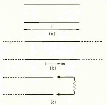
above:
Modification of Nyquist's method of deriving the formula for thermal
noise in a resistor.
First, consider a lossless transmission line of length I with both ends open-circuited as at (a) in the diagram. This will support standing-wave modes corresponding to integral numbers of half waves between the ends and hence 2l/delta-lambda modes in a wavelength interval 8X; and wavelengths are converted to frequencies according to the formula 1/lambda = f/c where c is the velocity of electromagnetic waves. Remembering that the open-circuit line behaves like an LC resonator with two degrees of freedom, so that it has equipartition energy of twice 1/2kT per mode, the energy in a limited frequency band 8 fin this line of length l is 2l sigma fkt/c. Now divide by l so as to give energy per unit length of line and then let line length tend to infinity, as represented at (b) in the diagram.
Two further points must be taken into account: firstly the power flowing along a line is energy density times velocity and secondly, each standing wave is the resultant of two travelling waves, one in each direction along the line. Since an infinite line is equivalent to a resistance equal to the characteristic impedance of the line, let the infinite line be cut in the neighborhood of the observer and one half discarded while the other half (still infinite, since infinity divided by two is still infinite) is terminated here by a matching resistor, as shown at (c) in the diagram. In thermal equilibrium the power flowing out of the line into the resistor must be equaled by the power flowing from the resistor into the line. In matched conditions the latter will be V2/4R, while the power flowing in one direction along the line is 84kT and equating these two gives the familiar Nyquist formula for squared noise voltage generated by a resistor,
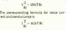
[The corresponding formula for noise current and conductance is...]
Objections to Nyquist's derivation have included: how do we know that there is thermal noise in an electrical circuit--answered by Johnson's experiment of heating a circuit--and can one visualize a truly loss-free and infinite line? With the development of superconductors one can have a resistance-free line, but even if there is no dielectric loss there will be a minute radiation resistance; and in fact some coupling with the surroundings, however small, is necessary to establish equipartition and is inherent in the assumption that the line can be observed.
The difficulty of infinite length is minimized by taking the energy per unit length (which Nyquist did not do) and the asymptotic approach to infinite length is to increase the length until the line appears to be perfectly matched by a resistor. The Nyquist model therefore appears to be reasonable.
Why did Nyquist not need to invoke quantum theory. as was necessary with black body radiation? In Nyquist's time the highest frequency used in electronic systems was such that hf was very small compared with kT, where h is Planck's constant and f the frequency. Under these conditions the Nyquist formula may be replaced by
P = kTB (2)
where P is the 'available power', i.e. the maximum power as delivered to a matched load, which for a source resistance R is V2/4R. and B for bandwidth replaces 81.
With the development of microwave frequencies and cryogenic devices, raising f and reducing T, it was thought necessary to add a quantum correction and a second formula was introduced:
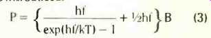
This included a half quantum, V2hf, which could not be exchanged with any real system and therefore was usually called "vacuum fluctuation". But it was shown by Bogo liubov and Shirkovs as early as 1951 that the average power is correctly given by the following formula:

P= hf coth( hf/kT)IB (4)
Series expansion of the exponential in (3) and of the hyperbolic cotangent in (4) shows that they are equivalent as far as the second power of hf/kT and to this degree of approximation they both modify (2) by a multiplier of 1 + (hf/kT)2/12. Only where temperature is very low and frequency is in gigahertz could one expect to detect any difference between (3) and (4).
The Nyquist formula can be applied to the real or resistive part of any impedance and, to complete the circle from breaking down the noise into a contribution per unit band width to finding the equipartition value of total noise (thermal) energy in an electric circuit, one can integrate from zero to infinity and find that the total voltage fluctuation has the value one would expect for the equipartition value of energy in the residual shunt capacitance which will be dominant at infinite frequency, 1/2CV2 = 1/2kT:
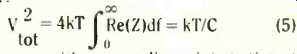
One can either use ordinary integration of the resistive part of a simple circuit such as R and C in parallel, or use contour integration of an arbitrary impedance, subject only to the condition that it reduces to a capacitance at infinite frequency. The latter method closely parallels some of the circuit integrals used by Bode. One can alternatively work in terms of current fluctuation and admittance to arrive at a total mean square fluctuation of current defined by 1/2LI^2 = 1/2kT, where L is the residual series inductance at infinite frequency.
SHOT NOISE
The second fundamental kind of noise, the second term in equation (1), is shot noise, which is found when electrons pass through a device randomly and independently. The prototype of shot noise was found in thermionic diodes in the absence of space charge, with electrons emitted from the cathode randomly and independently and passed practically instantaneously to the anode. Thermionic devices known as 'noise diodes' were at one time used as noise standards, but special precautions were needed to ensure the absence of space charge and of residual gas; and they could not be used at very low frequencies because of variations in cathode emission (flicker effect) or at very high frequencies at which the transit time of the electrons was significant. Shot noise was also found in vacuum photocells of the type in which electrons were released from the cathode by the impact of photons and collected by the anode.
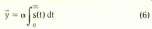
It was in connection with these devices that Rowland"' developed two theorems which can be used for shot noise and which are significant because they refer to the response of the apparatus to a pulse, not to the hypothetical current derived by spectral analysis of the pulses, a current which is then modified by the frequency response of the apparatus. If y is the output indication of measuring apparatus responding to events occurring randomly at a rate a per second and s(t) is the response of the apparatus to one such event, then the average output y, which we might identify as the DC component, is a times the response to one event:
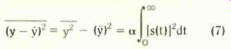
The mean square deviation, which we might identify with the noise as observed through an AC amplifier eliminating the DC, is a times the infinite integral of the square of the response to an individual event:
Now if the apparatus consists of a source of shot noise feeding current through a resistor shunted by a capacitor, s(t) for the sudden arrival of one electron is an instantaneous rise of voltage followed by an exponential decay of capacitor charge and voltage. But it might be asked how a single, indivisible, charge of one electron could decay exponentially.
The answer is that there will already be many electrons present so that the arrival of one more will only cause a perturbation of the distribution of electrons in the circuit, a perturbation which will decay exponentially.
The assumption of an exponential decay leads to agreement with another method of analysis and with experiment. Rowland's theorems present the noise as a time function, as did Kappler's mirror deflections records, so that the mean square value which they predict is, in our terms, the total noise, covering all frequencies.
An alternative method of calculating shot noise is to take the Fourier integral of a single electron transit, so as to obtain a spectrum, and assume that pulses occurring at random in time can be represented by spectral components in random phase which must be combined by summing squares of amplitudes. The result is that the mean square noise current per unit of bandwidth is
I^2 = 2Nq^2 (8a)
where N is the number of particles per unit time and q is the charge per particle. But charge x rate of arrival is equal to current, so on replacing q by e, if the particles are electrons, the shot noise current in band width df is
Idf^2 = 2iedf (8b)
The spectrum of the observed noise voltage will depend on the frequency characteristic of the circuit through which this current is passed.
THERMAL NOISE IN VALVES AND SOLID-STATE DEVICES
One of the first problems was to understand why the shot noise which was found in a thermionic device which was free from space charge was greatly reduced if space charge was present. This effect was known as space charge smoothing of shot noise and was important because all amplifying devices, such as valves with three or more electrodes, worked in a space-charge regime. (The mean-square smoothing factor was usually denoted by 1.2.) In 1938 the writer made the crude suggestion that the electron stream leaving the potential minimum (where most of the space charge was concentrated) could have a temperature, by analogy with the definable temperature of a flowing gas, and in a stream originating from thermionic emission and passing through a space charge barrier, a figure of half the cathode temperature was suggested". This was an over-simplification and a different approach by North 12 led to a factor of 0.644 times cathode temperature instead of a half. This is an asymptotic value which applies when the space charge is concentrated near the cathode; but in the transition between zero anode voltage and the asymptotic condition all the experimental results available in 1942 showed' that 1.2 was a function of the ratio eV/kT of energy supplied by the anode voltage to thermal energy from the cathode.
This is past history but it shows that thermal noise occurs in electron streams as well as in conductors.
In solid state devices shot noise is some times evident: it may be called 'injection noise' because one speaks of injection of electrons into a semiconductor instead of thermionic emission of electrons into a vacuum. But in general thermal noise pre dominates because the conduction electrons or holes collide with lattice atoms frequently enough to have a temperature related to the measurable temperature of the solid and may be said to be thermalized. So thermal noise can be minimized only by cooling the solid-state device to a low temperature, a method which would obviously be impossible with a device using thermionic emission, but which is particularly useful in earth stations for use with artificial satellites, because the background which the aerial 'sees' is outer space at a very low tempera ture. The limit on cooling of devices such as diodes, masers and parametric amplifiers is the cost of refrigeration; but there is also the SQUID which uses Josephson junctions between superconductors. Its name is an acronym for Superconducting Quantum interference Device.
NOISE IN SOLID-STATE DIODES AND TRIODES
The simplest solid-state device is the junction diode, but the complication is that it is a diffusion device in which electrons move in one direction and holes in the reverse direction and there is some recombination on the way, so that there is recombination noise as well as thermal noise. For forward bias it was shown by Van der Ziel 14 that the noise appears to depend on the sum of the actual diode current iD and twice the saturation reverse current is:
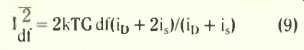
In the limit when iD is much greater than is the factor 2 instead of 4 in equation (9) may be taken as corresponding with the fact that the diode conducts for only half the time;
and when iD tends to zero, i.e. the diode has neither bias nor signal input, equation (9) can be reduced to the Nyquist form:
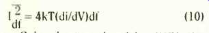
where C has been replaced by di/dV, the conductance of the diode.
The diode is a special case of a non-linear conductor, but general formulae for thermal noise in a conductor on any degree of non-linearity, provided it is in thermal equilibrium with its surroundings were given by Gupta in a review paper15, though if there is input of energy from any other source, e.g. electrical, arguments based on thermal equilibrium cease to be valid. A space-charge-limited solid-state device has a square-law relation between current and voltage, instead of the 3/2 law of a vacuum device, and for square-law devices, the thermal noise per unit bandwidth is doubled to 8kT times the differential resistance.
General non-linear devices may be treated by the salami method, in which the device is imagined to be cut into a stack of thin slices, each of which is treated as approximately linear and having a noise contribution which is therefore calculable by the Nyquist formula. The overall noise was originally found by summing squares of individual voltage contributions, but some modification is needed to take account of correlation, between slices, as proposed by Thornberth and implemented by Van Vliet et .3/.17. A theoretical difficulty with the salami method is that one is inclined to say "Let the slice thickness tend to zero and the summation of contributions be replaced by an integral." This cannot be correct in the limit because both the mean free path of electrons and the structure of the crystal introduce discontinuities when viewed on a small enough scale. A stratagem which seems legitimate is to interpolate a continuous curve through the discontinuities and integrate along the curve.
In 1960 the writer showed" that the transit of a single electron in vacuum between parallel plates produced a current in the external circuit while the electron was in transit, not merely when it arrived at the second plate. The idea of studying the effect on the external circuit of an electron moving within a device was generalized for solid state devices in 1966 by Shockley, Copeland and James" under the name of "field impedance method" with the important difference of dropping the assumption of continuity of electric current between the terminals. Because it relates current in the external circuit to movement of an electron at any point and in any direction in the device, the method is particularly suitable for calculating noise in Gunn effect devices, which depend on a domain of accelerated electrons moving between the terminals, since some of the noise current circulates within the domain but yet has an effect at the overall terminals. Since the method employs field integrals it meets the same difficulty as the salami method, namely integration through a fundamentally discontinuous structure, and this is overcome by substituting an approximating continuous function as integrand.
HOT ELECTRONS AND AVALANCHE AMPLIFICATION
A feature of solid-state conduction in semi conductors is that with small electric fields the result of frequent scattering by atoms of the solid is that the electrons, or holes, acquire a random component of velocity which can be regarded as representing a temperature equal to the temperature of the solid in which conduction is occurring. But if a sufficiently large electric field is applied, the random energy of the scattered electrons will exceed the thermal energy of the atoms of the solid; and the electrons are then said to be 'hot', since they have a higher equivalent temperature than their surroundings.
The effect of a sufficiently increased electric field is to cause liberation by impact of additional electrons from the atoms with which the primary electrons collide, leading to what is known as avalanche multiplication of the original current. (There are detailed factors which can make this process stable, in contrast to the destructive arc which may occur between metal electrodes in air.) A similar effect occurs in the vacuum types of photomultiplier which use secondary emission from intermediate anodes or from the wall of a narrow tube.
Now shot noise is proportional to the square of the charge carried per particle, so that if electrons arrive in groups of M, looking like single particles carrying M times the electron charge, the noise will be proportional to M^2. But the noise is further increased by the fact that M is only an average value, not a constant; and after taking account of the random variation in M the upper limit of increase in noise power is M^3 for large values of avalanche multiplication. The signal current is multiplied by M and signal power by M^2, so the signal-to noise power ratio is deteriorated by a factor not greater than M. the ratio by which current is amplified by avalanche.
SPECIAL TYPES OF FET
At the present time, special interest attaches to transistors for use at frequencies of a few tens of GHz up to 100 GHz. One may hope for ballistic transport, which means that electrons shoot through the device without collision and scattering, thus eliminating thermal noise at the temperature of the semiconductor but leaving shot (or injection) noise. One can raise mobility, presumably raising the mean free path, (at the present time it is not practicable to make a FET with gate length much less than a quarter of a micrometer) by transfer of electrons between gallium-aluminum-arsenide and gallium arsenide to make a high-electron-mobility transistor. This is referred to by the initials h.e.m.t. and is identical in structure with a mosfet, which is a field-effect transistor in which the doping is modulated, i.e. varied from one part to another. It has been stated by Duh el al.2" that this type of FET is suitable for millimeter waves and has shown the lowest noise figure yet recorded up to 62 CHz, where it is 2.7 decibels.
1/f NOISE
The foregoing allows one to calculate the noise (thermal and shot) at frequencies above the lower limit at which the phenomenon of 1/f noise predominates. This is usually below 1 kHz and may be as low as tens of Hertz, though in point contacts 1/f noise has been found in the MHz range: and it arises only when a steady current flows, the 1/f noise power being proportional to the square of the steady current.
The feature which makes 1/f noise so difficult theoretically is the absence of any detectable lower limit to the inverse frequency law. In one of the earlier experiments Rollin and Templeton recorded noise from resistors consisting of pyrolytic carbon films on magnetic tape running 800 to 80,000 times more slowly than normal and performed a frequency analysis of the output from the tape when running at normal speed. After applying a correction for the frequency characteristic of the tape recorder they found a close fit to a 1/f law from 5.10' to 8 Hz. The line to which the points fitted closely was represented by the formula sigma R2/R2 = 10^-13df/f which expresses the noise as the square of a fluctuation in resistance.
This is a natural form to adopt since the squared noise voltage is proportional to the square of voltage due to the steady current, V- = i^2R^2. This idea of fluctuation of resistance as the source of 1/f noise has been widely used but it has been challenged and must not be taken as evidence of the source of 1/f noise.. Later work on silicon by Caloyannides has extended the spectrum down to le Hertz and by piecing together the results of various experiments one can demonstrate a 1/f law over at least ten decades. which is ten thousand million to one in frequency.
It has been suggested that the law might not be 1/f but one upon the square root of a2 + (2, which would give 1/f for large f, but a flat spectrum for very low frequencies where (2 is much smaller than a2. But although this is mathematically more reasonable, there has never been any experimental evidence of a lower limit to a 1/f spectrum.
The problem is complicated by the occurrence of a 1/f law in a wide variety of non-electrical phenomena where it might be described qualitatively as a general rule that "the bigger the fewer". In electronics the first doubt was whether the extrapolation of 1/f to zero frequency posed a problem of infinite power similar to the ultra-violet catastrophe predicted by the application of classical equipartition theory to black body radiation, but it was pointed out by Flinn that the effect was so small that the 1/f noise power in a resistor, over any conceivable frequency range and taking the age of the universe as the period of the lowest frequency, would be only a small fraction of the power input from the steady current which excited the noise.
Early theories that 1/f noise was associated with contacts through which the exciting current was fed to the device have been ruled out by the use of four-terminal experimental bodies, so that the contacts through which current is injected are not included in the circuit in which noise is measured. One of the conventional ideas, proposed by Van de Ziel in 1950, was that the l/t law was approximated by a collection of phenomena having spectra of the form 1/(a2- r2). but with the values of a2 and the weighting of individual components so spread that the combination of the flat parts of the spectra for small f and 1/f^2 for large f would produce 1/f in an intermediate range of frequencies.
The objections to this are firstly that the predicted flat spectrum at small enough f has never been found experimentally and secondly that the range of values of a- must be twice the range of frequencies over which 1/f is to apply. It is difficult to envisage a mechanism which would both have a correctly weighted range of time-constants of twenty decades (taking the experimentally observed range of the 1/f law as ten decades) and be found in all the substances and systems in which the 1/f law has been found.
In 1969 Hooge25 showed that most of the experimental results in silicon were consistent with the 1/f noise being inversely proportional to the number of electrons involved in the conduction, according to the formula
...and he suggested that sigma was a universal constant having the approximate value 2.10^-3. Later results from other materials were not consistent with 8 having a universal value, so formula (11) was modified by Hooge et a/.26 who proposed in 1979 that only scattering by the crystal lattice, not as surface or other irregularities, was relevant, thus arriving at equation (12):
a = (114titt)-ao (12)
The total scattering was apportioned between the lattice and other scattering mechanisms by representing scattering as inversely proportional to mobility, the total value of which can be measured. The correction factor in (12) is necessarily less than unity, so it would account for values of a less than that found originally in silicon.
Kleinpennine has related 1/f noise to fluctuations in mobility. This would not be inconsistent with the relation to lattice scattering when this is expressed through its effect on mobility, nor with the overall expression as a resistance fluctuation.
However, the mechanism which produces the 1/f shape of spectrum has still to be explained, especially as 1/f noise is found in so many different materials and phenomena.
Throughout the history of 1/f noise, now over 50 years. there has been controversy as to whether it arises in the bulk of the conductor or only at surfaces unfortunately the answer seems to be both, so one might be forced to assume that there is more than one mechanism. The only rules for minimizing 1/f noise in practice are first, to use as large a body as possible so as to maximize the number of electrons participating in conduction; second, to avoid concentration of steady current in narrow paths because the noise is proportional to the square of current density; third, to minimize defects such as surface leakage, impurities or other defects in crystal structure; or fourth, to avoid 1/f noise entirely by using a modulation scheme to eliminate low frequencies. Other design considerations, such as miniaturization, may be opposed to some of these rules, but as long as 1/-f noise remains a mystery, the only conclusive rule is to avoid the use of very low frequencies as far as possible.
The substance of this article is available as a two-part lecture on video tape. Copies may be obtained from the Audio-Visual Centre, University of Hull, Hull HU6 7RX.
References
1. Shannon. C.E., 1948. A Mathematical Theory of Communication. Bell Syst. Tech. J..27 379-423 and 623-656.
2. Haldane, J.B.S. (Editor) 1928. The Collected Scientific Papers of J.J. Waterston. (Oliver & Boyd, Edinburgh.)
3.Kappler, E., 1931. Versuche zur Messung der Avogadro-Loschmidtschen Zahl aus der Brown sche Bewegung einer Drehwaage. Ann. d. Phys 11. 233-256.
4. Callen, H.R. and Welton, TA., 1951. Irreversibility and Generalized Noise. Phys. Rev. 83.34-40.
5. Johnson. J.B. 1928. Thermal Agitation of Electricity in Conductors. Phys. Rev. 32, 97-109.
6. Rayleigh, Lord, 1900. Remarks upon the Law of Complete Radiation Phil. Mag. 49. 539-540.
7. Nyquist, H., 1928. Thermal Agitation of Electric Charge in Conductors. Phys. Rev. 32, 110-113.
8. Bogoliobov, N.N. and Shirkov, D.V., 1959. Introduction to the Theory of Quantized Fields. (lnterscience Publishers Ltd, London.)
9. Bode. H.W. 1945. Network Analysis and Feed back Amplifier Design. ( Van Nostrand, New York.)
10. Rowland, E.N., 1936. The Theory of the Mean Square Variation of a Function formed by adding known Functions with Random Phases, and applications to the Theories of the Shot Effect and of Light. Proc. Camb. Phil. Soc., 32, 580-597.
11. Bell, DA.. 1938. A Theory of Fluctuation Noise. J.IEE 82, 522-536.
12. North, D.O., 1940. Fluctuations in Space-charge-limited Currents at Moderately High Frequencies. RCA Rev., 5.244-260.
13. Bell. DA., 1942. Fluctuations in Space-charge-limited Currents. J.IEE. 89 Part III. 207 212.
14. Van der Ziel, A., 1970. Noise in Solid-state Devices and Lasers. Proc. IEEE. 58. 1178-1206.
15. Gupta, M.S., 1982. Thermal Noise in Non linear Resistive Devices and its Circuit Representation. Proc. IEEE, 70, 788-804.
16. Thomber. K.K., 1974. Some Consequences of Spatial Correlation on Noise Calculation, Solid St. Electronics, 17, 95-97.
17. Van Vliet, K.M., Friedman, A., Zifistra, RJ.J., Gisolf, A. and Van der Ziel. A.. 1975. Noise in Single Injection Diodes. J. Appl., Phys.. 46. 1804 1823.
18. Bell, DA., 1960. Electrical Noise. (Van Nostrand, London).
19. Shockley, W., Copeland, JA. and James, R.P.. 2966. The impedance field method of noise calculation in active semiconductor devices in Quantum theory of atoms, molecules and the solid state, Ed. Per-Olav Lowdin (Academic Press, London).
20. Duh, K.H.G.. Chao, P.C., Smith, P.M., Lester L.F. and Lee. B.R., 1986. 60 GHz Low-noise High-Electron-Mobility Transistors. Electronics Letters, 22.647-649.
21. Rollin, B.V. and Templeton, I.M., 1953. Noise in Semiconductors at Very Low Frequencies. Proc. Phys. Soc. B, 66.259-261.
22. Caloyannides, MA., 1974, Microcycle Spectral Estimates of I/f Noise in Semiconductors. J. Appl. Phys.. 45, 307-316.
23. Flinn, I., 1968. Extent of the 1/f noise spectrum. Nature, 219. 1356-1357.
24. Van der Ziel, A., 1950. On the Noise Spectra of Semiconductor Noise and of Flicker Effect. Physics, 16, 359-372.
25. Hooge. F.N., 1969. I/f Noise is No Surface Effect. Phys. Lett. A, 29, 139-140.
26. Hooge. F.N., Kedzia, J. and Vandamme. L.K.J., 1979. Boundary Scattering and I/f Noise. J. Appl. Phys., 50, 8087-8089.
27. Kleinpenning, T.G.M., 1986. On I/f Mobility Fluctuations in Bipolar Transistors. Physics, 138 B+C. 244-252.
==========
(adapted from: Wireless World , Dec. 1987)