AMAZON multi-meters discounts AMAZON oscilloscope discounts
Objectives
This Section is an introduction to different process control concepts and will help you understand and become familiar with the different process control actions.
The topics covered in this Section are as follows:
_ Concepts of signal control and controller modes
_ Concept of lag time, error signals, and correction signals
_ ON/OFF types of process controller action
_ Proportional, derivative, and integral action in process controllers
_ ON/OFF pneumatic control systems
_ ON/OFF electric controllers
_ Pneumatic proportional, integral, and derivative (PID) controllers
_ Analog electronic implementation of proportional, derivative, and integral action
_ An electronic PID loop
_ Digital controller system
1. Introduction
Control systems vary extensively in complexity and industrial application. Industrial controllers, for instance, in the petrochemical industry, automotive industry, soda processing industry, and the like, have completely different types of control functions. The control loops can be very complex, requiring micro processor supervision, down to very simple loops such as those used for con trolling water temperature or heating, ventilation, and air-conditioning (HVAC) for comfort. Some of the functions need to be very tightly controlled, with tight tolerance on the variables and a quick response time, while in other areas the tolerances and response times are not so critical. These systems are closed loop systems. The output level is monitored against a set reference level and any difference detected between the two is amplified and used to control an input variable which will maintain the output at the set reference level.
2. Basic Terms
Some of these terms have already been defined, but apply to this Section. Hence, the terms are redefined here for completeness.
Lag time is the time required for a control system to return a measured vari able to its set point after there is a change in the measured variable, which could be the result of a loading change or set point change and so on.
Dead time is the elapse time between the instant an error occurs and when the corrective action first occurs.
Dead-band is a set hysteresis between detection points of the measured vari able when it is going in a positive or a negative direction. This band is the separation between the turn ON set point and the turn OFF set point of the controller and is sometimes used to prevent rapid switching between the turn ON and turn OFF points.
Set point is the desired amplitude of an outpoint variable from a process.
Error signal is the difference between a set reference point and the amplitude of the measured variable.
Transient is a temporary variation of a load parameter after which the parameter returns to its nominal level.
Measured variable is an output process variable that must be held within given limits.
Controlled variable is an input variable to a process that is varied by a valve to keep the output variable (measured variable) within its set limits.
Variable range is the acceptable limits within which the measured variable must be held and can be expressed as a minimum and a maximum value, or a nominal value (set point) with ± spread (percent).
Control parameter range is the range of the controller output required to control the input variable to keep the measured variable within its acceptable range.
Offset is the difference between the measured variable and the set point after a new controlled variable level has been reached. It is that portion of the error signal which is amplified to produce the new correction signal and produces an "Offset" in the measured variable.
3. Control Modes
The two basic modes of process control are ON/OFF action and "continuous control" action. In either case the purpose of the control is to hold the measured variable output from a process within set limits by varying the controlled input variable to the process.
In the case of ON/OFF control (discrete control or two position control), the output of the controller changes from one fixed condition (ON) to another fixed position (OFF). Control adjustments are the set point and in some applications a dead-band is used. In continuous control (modulating control) action the feed back controller determines the error between a set point and a measured vari able. The error signal is then used to produce an actuator control signal to operate a valve and reduce the error signal. This type of control continuously monitors the measured variable and has three modes of operation which are proportional, integral, and derivative. Controllers can use one of the functions, two, or all three of the functions as required.
3.1 ON/OFF action
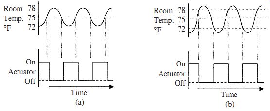
FIG. 1 A room heating system with (a) simple ON/OFF action of a room
heating system and (b) differential ON/OFF action.
The simplest form of control in a closed loop system is ON/OFF action. The measured variable is compared to a set reference. When the variable is above the reference the system is turned ON and when below the reference the system is turned OFF or vice versa, depending upon the system design. This could make for rapid changes in switching between states. However, such systems normally have a great deal of inertia or momentum which produces over-swings and introduces long delays or lag times before the variable again reaches the reference level.
FIG. 1a shows an example of a simple room heating system. The top graph shows the room temperature or measured variable and the lower graph shows the actuator signal. The room temperature reference is set at 75°F. When the air is being heated, the temperature in the center of the room has already reached 77°F before the temperature at the sensor reaches the reference temperature of 75°F and similarly as the room cools, the temperature in the room will drop to 73°F before the temperature at the sensor reaches 75°F. Hence, the room temperature will go from about 72°F to 78°F due to the inertia in the system.
3.2 Differential action
Differential or delayed ON/OFF action is a mode of operation where the simple ON/OFF action has hysteresis or a dead-band built in. FIG. 1b shows an example of a room heating system similar to that shown in Fig. 1a except that instead of the thermostat turning ON and OFF at the set reference of 75°, the switching points are delayed by ±3°F. As can be seen in the top graph, the room temperature reaches 78°F before the thermostat turns OFF the actuator and the room temperature falls to 72°F before the actuator is turned ON giving a built in hysteresis of 6°F. There is, of course, still some inertia. Hence, the room temperature will go from about 70°F to about 80°F.
3.3 Proportional action
The most common of all continuous industrial process control action is proportional control action. The amplitude of the output variable from a process is measured and converted to an electrical signal. This signal is compared to a set reference point. Any difference in amplitude between the two (error signal) is amplified and fed to a control valve (actuator) as a correction signal. The control valve controls one of the inputs to the process. Changing this input will result in the output amplitude changing until it is equal to the set reference or the error signal is zero. The amplitude of the correction signal is transmitted to the actuator controlling the input variable and is proportional to the percentage change in the output variable amplitude measured with respect to the set reference. In industrial processing a different situation exists than with a room heating system. The industrial system has low inertia; overshoot and response times must be minimized for fast recovery and to keep processing tolerances within tight limits. In order to achieve these goals fast reaction and settling times are needed. There may also be more than one variable to be controlled and more than one output being measured in a process.
The change in output level may be a gradual change, a large on-demand change, or caused by a change in the reference level setting. An example of an on-demand change would be cleaning stations using hot water at a required fixed temperature, as shown in Fig. 2a. At one point in time the demand could be very low with a low flow rate as would be the case if only one cleaning station were in use. If cleaning commenced at several of the other stations, the demand could increase in steps or there could be a sudden rise to a very high flow rate.
The increased flow rate would cause the water temperature to drop. The drop in water temperature would cause the temperature sensor to send a correction signal to the actuator controlling the steam flow, so as to increase the steam flow to raise the temperature of the water to bring it back to the set reference level (see Fig. 2b). The rate of correction will depend on the inertia in the system, gain in the feedback loop, allowable amount of overshoot, and so forth.
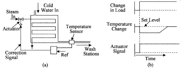
FIG. 2 Water heater (a) showing a feedback loop for constant temperature
output and (b) effect of load changes on the temperature of the water from
the water heater.
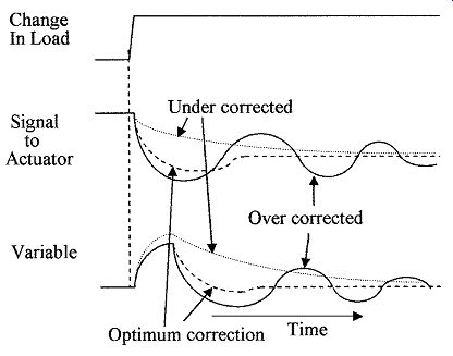
FIG. 3 Effect of loop gain on correction time using proportional action
with over correction and under correction.
In a closed loop feedback system settings are critical. If the system has too much gain, i.e., the amplitude of the correction signal is too great, it will cause the controlled variable to over correct for the error, which in turn will give a false error signal in the reverse direction. The actuator will then try to correct for the false error signal. This can, in turn, send a larger correction signal to the actuator, which will cause the system to oscillate or cause an excessively long settling or lag time. If the gain in the system is too low the correction signal is too small and the correction will never be fully completed, or again an excessive amount of time is taken for the output to reach the set reference level.
This effect is shown in Fig. 3 (a), as can be seen in comparing the over corrected (excessive gain) and the under corrected (too little gain) to the optimum gain case (with just a little overshoot). The variable takes a much longer time for the correction to be implemented than in the optimum case. In many processes this long delay or lag time is unacceptable.
3.4 Derivative action
Proportional plus derivative (PD) action was developed in an attempt to reduce the correction time that would have occurred using proportional action alone.
Derivative action senses the rate of change of the measured variable and applies a correction signal that is proportional to the rate of change only (this is also called rate action or anticipatory action). FIG. 4a shows some examples of derivative action. As can be seen in this example, a derivative output is obtained only when the load is changing. The derivative of a positive slope is a positive signal and the derivative of a negative slope is a negative signal; zero slopes give zero signals as shown. An in-depth look at derivatives is outside the scope of this text.
FIG. 4b shows the effect of PD action on the correction time. When a change in loading is sensed as shown, both the proportional and derivative signals are generated and added. The significance of combining these two signals is to produce a signal that speeds up the actuator's control signal. The faster reaction time of the control signal reduces the time to implement corrective action reducing the excursion of the measured variable and its settling time. The amplitudes of these signals must be adjusted for optimum operation, or over shoot or under shoot can still occur.
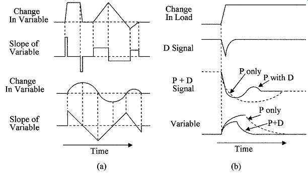
FIG. 4 Proportional and derivative action (a) variable change with
resulting slope and (b) effect of proportional and derivative action on
a variable.
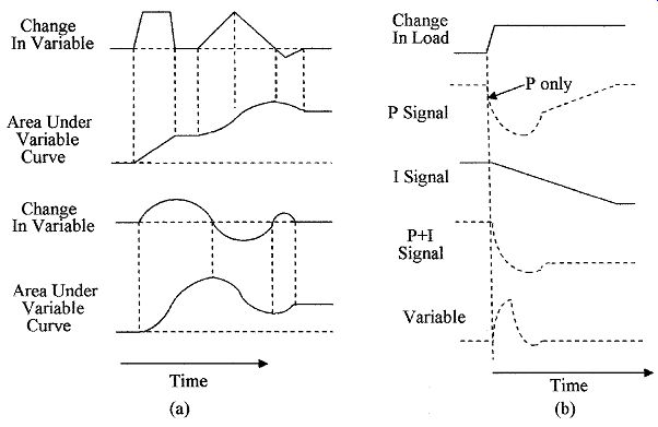
FIG. 5 Proportional and integral action (a) variable change with area
under the graph and (b) effect of proportional and integral action on a
variable.
3.5 Integral action
Proportional plus Integral (PI) action also known as reset action, was developed to correct for long-term loads and applies a correction proportional to the area under the change in the variable curve. FIG. 5a gives some examples of the integration of a curve or the area under a curve. In the top example the area under the square wave increases rapidly but remains constant when the square wave drops back to zero. In the triangular section the area increases rapidly at the apex but increases slowly as the triangle approaches zero; when the triangle goes negative, the area reduces. In the lower example the area increases more rapidly when the sine wave is at its maximum and slower as it approaches the zero level. During the negative portion of the sine wave, the area is reduced.
Proportional action gives a response to a change in the measured variable but does not fully correct the change in the measured variable due to its limited gain.
For instance, if the gain in the proportional amplifier is 100, then when a change in load occurs, 99 percent of the change is corrected. However, a 1 percent error signal is required for amplification to drive the actuator to change the manipulated variable. The 1 percent error signal is effectively an "offset" in the vari able with respect to the reference. Integral action gives a slower response to changes in the measured variable to avoid overshoot, but has a high gain so that with long-term load changes it takes over control of the manipulated variable and applies the correction signal to the actuator. Because of the higher gain the measured variable error is reduced to close to zero. This also returns the proportional amplifier to its normal operating point, so that it can correct for other fluctuations in the measured variable. Note that these corrections are done at relatively high speeds. The older pneumatic systems are much slower and can take several seconds to make such a correction. FIG. 5b shows the PI corrective action waveforms. When a change in loading occurs, the P signal responds to take corrective action to restore the measured vari able to its set point; simultaneously, the integral signal starts to change linearly to supply the long term correction, thus allowing the proportional signal to return to its normal operating point as is shown. Here again integral action can become complex and further discussion is considered to be outside the scope of this text.
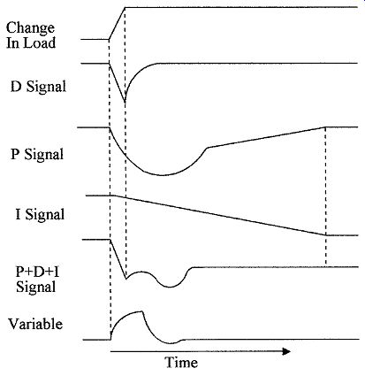
FIG. 6 Waveforms for proportional plus integral action and waveforms
for proportional plus derivative and integral action.
3.6 PID action
A combination of all three of the actions described above is more commonly referred to as PID action. The waveforms of PID action are illustrated in Fig. 6.
PID is the most often used corrective action for process control. There are how ever, many other types of control actions based upon PID action. Understanding the fundamentals of PID action gives a good foundation for understanding other types of controllers. The waveforms used have been idealized for ease of the explanation and are only an example of what may be encountered in practice.
Loading is a function of demand and is not affected by the control functions or actions; the control function is to ensure that the variables are within their specified limits.
To give an approximate indication of the use of PID controllers for different types of loops, the following are general rules that should be followed:
Pressure control requires proportional and integral; derivative is normally not required.
Level control uses proportional and sometimes integral, derivative is not normally required.
Flow control requires proportional and integral; derivative is not normally required.
Temperature control uses proportional, integral, and derivative usually with integral set for a long time period.
However, the above are general rules and each application has its own requirements.
Typical feedback loops have been discussed. The reader should, however, be aware that there are other kinds of control loops used in process control such as cascade, ratio, and feed-forward.
4. Implementation of Control Loops
Implementation of the control loops can be achieved using pneumatic, analog, or digital electronics. The first process controllers were pneumatic. However, these have largely been replaced by electronic systems, because of improved reliability, less maintenance, easier installation, easier adjustment, higher accuracy, lower cost, can be used with multiple variables, and have higher speed operation.
4.1 ON/OFF action pneumatic controller
FIG. 7 shows a pneumatic furnace control system using a pneumatic ON/OFF controller. In this case the furnace temperature sensor moves a flap per that controls the air flow from a nozzle. When the temperature in the furnace reaches its set point the sensor moves the flapper toward the nozzle to stop the air flow and allow pressure to build up in the bellows. The bellows operates an air control relay that shuts OFF the air flowing to the control valve turning OFF the fuel to the furnace. When the temperature in the furnace drops below a set level the flapper is opened by the sensor, reducing the air pressure in the bellows, which in turn opens the air control valve allowing the air pressure to drop and the control valve to open, turning ON the fuel to the furnace.
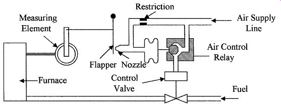
FIG. 7 Pneumatic ON/OFF furnace controller.
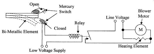
FIG. 8 Simple ON/OFF room heating controller.
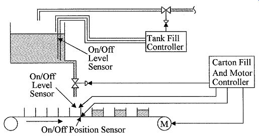
FIG. 9 Example of the use of ON/OFF controls used for carton filling.
4.2 ON/OFF action electrical controller
An example of an ON/OFF action electrical room temperature controller is shown in Fig. 8. In this case the room temperature is sensed by a bimetallic sensor. The sensor operates a mercury switch. As the temperature decreases the bimetallic element tilts the mercury switch down causing the mercury to flow to the end of the glass envelope and in so doing shorts the two contacts together in the mercury switch. The contact closure operates a low voltage relay turning ON the blower motor and the heating element. When the room temperature rises to a predetermined set point the bimetallic strip tilts the mercury switch back causing the mercury to flow away from the contacts. The low voltage electrical circuit is turned OFF, the relay opens, and the power to the heater and the blower motor is disconnected.
The ON/OFF controller action has many applications in industry; an example of some of these uses is shown in Fig. 9. In this case, cartons on a conveyer belt are being filled from a hopper. When a carton is full it is sensed by the level sensor, which sends a signal to the controller to turn OFF the material flowing from the hopper and to start the conveyer moving. As the next carton moves into the filling position it is sensed by the position sensor, which sends a signal to the controller to stop the conveyer belt and to start filling the carton. Once it is full the cycle repeats itself.
A level sensor in the hopper senses when the hopper is full and when it is almost empty. When empty, the sensor sends a signal to the controller to turn ON the feed valve to the hopper and when the hopper is full it is detected and a signal is sent to the controller to turn the feed to the hopper OFF.
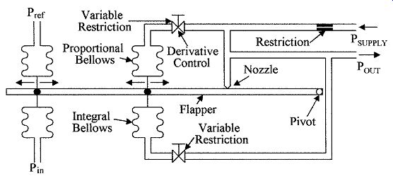
FIG. 10 Pneumatic PID controller.
4.3 PID action pneumatic controller
Many configurations for PID pneumatic controllers have been developed over the years, have served us well, and are still in use in some older processing plants.
But pneumatic controllers have, with the advent of the requirements of modern processing and the development of electronic controllers, achieved the distinction of becoming museum pieces. FIG. 10 shows an example of a pneumatic PID controller. The pressure from the sensing device Pin is compared to a set or reference pressure Pref to generate a differential force (error signal) on the flapper to move the flapper in relation to the nozzle giving an output pressure proportional to the difference between Pin and Pref. If the derivative restriction is removed the output pressure is fed back to the flapper via the proportional bellows to oppose the error signal and to give proportional action. System gain is adjusted by moving the position of the bellows along the flapper arm, i.e., the closer the bellows is positioned to the pivot the greater the movement of the flapper arm.
By putting a variable restriction between the pressure supply and the proportional bellows, a change in Pin causes a large change in Pout, as the feedback from the proportional bellows is delayed by the derivative restriction. This gives a pressure transient on Pout before the proportional bellows can react, thus giving derivative action. The duration of the transient is set by the size of the bellows and the setting of the restriction.
Integral action is achieved by the addition of the integral bellows and restriction as shown. An increase in Pin moves the flapper towards the nozzle causing an increase in output pressure. The increase in output pressure is fed to the integral bellows via the restriction until the pressure in the integral bellows is sufficient to hold the flapper in the position set by the increase in Pin, creating integral action.
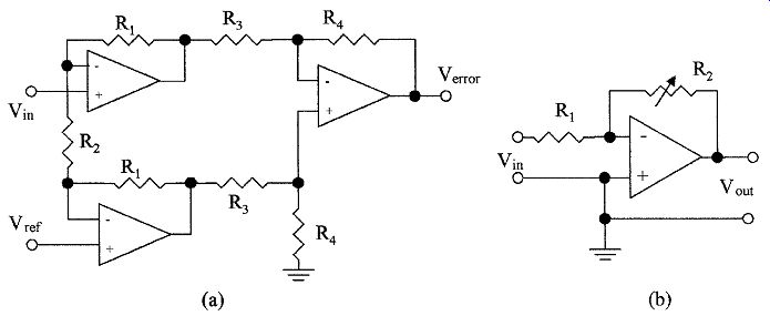
FIG. 11 Circuits used in PID action (a) error generating circuit and
(b) proportional circuit.
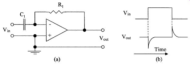
FIG. 12 Derivative amplifier (a) circuit and (b) waveforms.
4.4 PID action control circuits
PID action can be performed using either analog or digital electronic circuits. In order to understand how electronic circuits are used to perform these functions, the analog circuits used for the individual actions will be discussed. The circuit shown in Fig. 11a is used to compare the signal from the measured variable and the reference to generate the error signal. Proportional action is achieved as shown in Fig. 11b by amplifying the error signal Vin. The stage gain is the ratio of R2/R1; the gain can be adjusted using the potentiometer R2. The output is inverted.
The circuit for derivative action is shown in Fig. 12a. The feedback resistor can be replaced with a potentiometer to adjust the differentiation duration.
The output signal is inverted. This signal can be changed to a noninverted signal with an inverting amplifier stage if required. The waveforms of the differentia tor are shown in Fig. 12b.
Proportional and derivative action can be combined using the circuit shown in Fig. 13a. Derivative action is obtained by the input capacitor C1 and proportional action by the ratio of the resistors R1 and R2. The inverted output signal is shown in Fig. 3b.
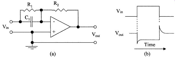
FIG. 13 Proportional plus derivative amplifier (a) circuit and (b)
waveforms.
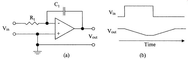
FIG. 14 Integrating amplifier (a) circuit and (b) waveforms.
A circuit to perform integral action is shown in Fig. 14a. Capacitive feed back around the amplifier prevents the output from the amplifier from following the input change. The output changes slowly and linearly when there is a change in the measured variable as shown in the waveforms in Fig. 14b. The slope of the output waveform is set by the time constant of the feedback C1 and the input resistance R . This is integral action and the output from the integrator is the area under the input waveform. This area can be adjusted by replacing R1 with a potentiometer. The output of the amplifier is inverted.
4.5 PID electronic controller
FIG. 15 shows the block diagram of an analog PID controller. The measured variable from the sensor is compared to the set point in the first unity gain comparator; its output is the difference between the two signals or the error signal. This signal is fed to the integrator via an inverting unity gain buffer and to the proportional amplifier and differentiator via a second inverting unity gain comparator, which compares the error signal to the integrator output. Initially, with no error signal the output of the integrator is zero so that the zero error signal is also present at the output of the second comparator.
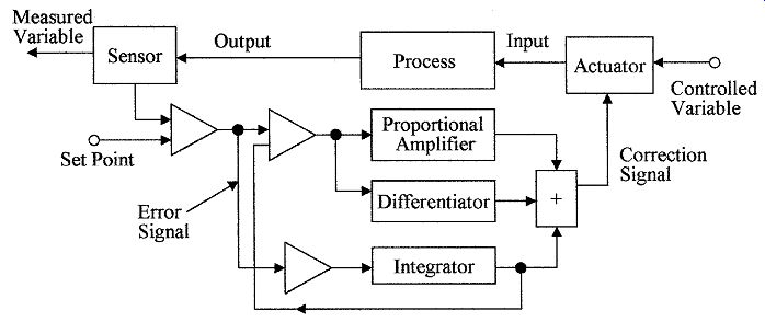
FIG. 15 Block schematic of a PID electronic controller.
When there is a change in the measured variable, the error signal is passed through the second comparator to the proportional amplifier and the differentiator where it is amplified in the proportional amplifier, added to the differential signal in a summing circuit, and fed to the actuator to change the input variable. Although the integrator sees the error signal, it is slow to react and so its output does not change immediately, but starts to integrate the error signal.
If the error signal is present for an extended period of time, the integrator will supply the correction signal via the summing circuit to the actuator and input the correction signal to the second comparator. This will reduce the effective error signal to the proportional amplifier to zero, when the integrator is sup plying the full correction signal to the actuator. Any new change in the error signal will still be passed through the second comparator as the integrator is only supplying an offset to correct for the first long-term error signal. The proportional and differential amplifiers can then correct for any new changes in the error signal.
The circuit implementation of the PID controller is shown in Fig. 16. This is a complex circuit because all the amplifier blocks are shown doing a single function to give a direct comparison to the block diagram and is only used as an example. In practice there are a large number of circuit component combi nations that can be used to produce PID action.
A single amplifier can also be used to perform several functions which would greatly reduce the circuit complexity. Such a circuit is shown in Fig. 17, where feedback from the actuator position is used as the proportional band adjustment.
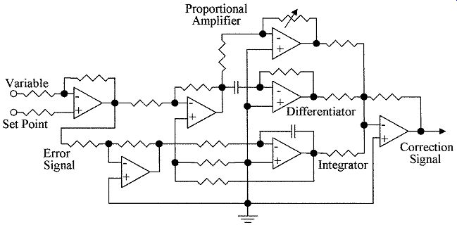
FIG. 16 Circuit of a PID action electronic controller.
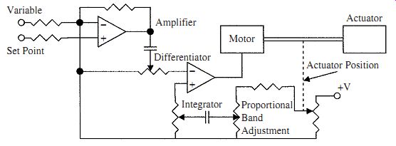
FIG. 17 Circuit of a PID electronic controller with feed back from
the actuator position.
In new designs, PLC processors can be used to replace the analog circuits to perform the PID functions using digital techniques.
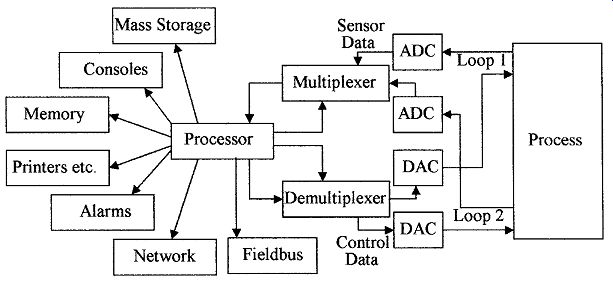
FIG. 18 Computer based digital controlled process.
5. Digital Controllers
Modern process facilities will use a computer or PLC processor as the heart of the control system. The system will be able to control analog loops, digital loops, and will have a foundation fieldbus input/output for communication with smart sensors. All of these control functions may not be required in small process facilities but in large facilities they are necessary. The individual control loops are not independent in a process but are interrelated and many measured variables may be monitored and manipulated variables controlled simultaneously. Several processors may also be connected to a mainframe computer for complex control functions. FIG. 18 shows the block diagram of a processor controlling two digital loops. The analog output from the monitors is converted to a digital signal in an ADC. The loop signal is then selected in a multiplexer and PID action is performed in the processor using software pro grams. The digital output signal is then fed to the actuator through a demultiplexer and a DAC. The processor has mass storage for storing process data for later use or making charts and graphs and will also be able to control a number of peripheral units and monitors as shown.
Digital controllers will compare the digitized measured variable to the set point stored in memory to produce an error signal which it can amplify under program control and feed to an actuator via a DAC. The processor can measure the rate of change of the measured variable and produce a differential signal to add to the digital correction signal. In addition, the processor can measure the area under the measured variable signal which it will also add to the digital correction signal. All of these actions are under program control; the setting of the program parameters can be changed with a few key strokes, making the system much more versatile than the analog equivalent.
Summary
This Section discussed process control and the various methods of implementation of the controller functions. Various controller modes and the methods of implementing the modes in pneumatic and electronic circuits are described. Understanding of these circuits will enable the reader to extend these principles to other methods of control.
The salient points covered in this section were:
1. ON/OFF and delayed ON/OFF action and their use in HVAC. A number of examples of ON/OFF action in process control were given.
2. Proportional, integral, and derivative action and their use in process control. The effects of gain setting in proportional control.
3. Circuits to perform proportional, integral, differential action and methods of combining the various actions in a PID controller are described.
4. The operation of pneumatic controller actions using flappers, nozzles, and bel lows combinations is given. A combination of the various pneumatic components is used to make a PID controller.
5. Digital controller concepts in modern processing facilities are given.
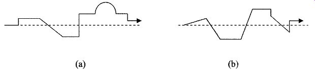
FIG. 19 Change in measured variable for Prob. 6 through 9.
Problems
1. Describe controller ON/OFF action.
2. What is the difference between simple ON/OFF action and differential ON/OFF action?
3. What is proportional action?
4. What is integral action?
5. What is derivative action?
6. Draw the derivative signal for the variable shown in Fig. 19a.
7. Draw the integral signal for the variable shown in Fig. 19a.
8. Draw the derivative signal for the variable shown in Fig. 19b.
9. Draw the integral signal for the variable shown in Fig. 19b.
10. Redraw the PID action controller in Fig. 16 as it would be if integral action was not required.
11. Give a list of applications for ON/OFF controller action.
12. Why is the gain setting critical in proportional action?
13. What is the difference between an error signal and a measured variable signal?
14. What is the difference between lag time and dead time?
15. What is the difference between offset and error signal?
16. What are some of the actions that can be taken to reduce correction time?
17. What is a dead-band?
18. What would be the effect of time constants on correction time?
19. What types of control do not normally require derivative action?
20. Why is ON/OFF action not normally suitable for control of a process?
Related Articles -- Top of Page -- Home