Position and Motion Sensors

1. Contact and Non-contact Position Sensors

Introduction

Position sensors play an increasing role in our daily lives. They are abundant in our homes, in our cars, and in our work places. As sensing technology improves, positioning devices continue to get smaller, better and more inexpensive, opening the way for more applications than ever before.

As their name implies, position sensors provide position feedback. They are able to perform precise motion control, encoding and counting functions by determining the presence or absence of a target or by detecting its motion, speed, direction or distance.

Position sensors detect a target object, a person, a substance or the disturbance of a magnetic or an electrical field and convert that physical parameter to an electrical output to indicate the target's position.

There are many ways to sense the position of a target. Some of them, such as limit switches and potentiometers, involve physical contact with the object being sensed.

These are called contact position sensors. Contact position sensors often prove to be the simplest, lowest cost solution in applications where contact with the target is acceptable.

Sensor manufacturers have employed a much wider variety of approaches and technologies to develop non-contact position sensors, which have no physical contact with target objects and don't "wear out" from repeated contact. This SECTION does not cover every possible technology that can be applied to sense position. The aim here is to provide a good understanding of the most commonly used technologies and the reasons one technology might be preferred over another in specific applications.

Types of Position Sensors

Every commonly applied position sensing technology has its own characteristic benefits and limitations. Obviously, some of these technologies provide a better fit than others in different applications. The goal is to find the most cost-effective solution for the performance parameters that are important in your specific application and environment. The types of position sensors covered here include:

¦ Contact devices

• Limit switches

• Resistive position transducers

¦ Non-contact devices

• Magnetic sensors, including Hall effect and magneto-resistive sensors

• Ultrasonic sensors

• Proximity sensors

• Photoelectric sensors

Limit Switches

Limit switches are electromechanical contact devices. Easy to understand and apply, they are the cost-effective switches of choice for detecting objects that can be touched. These rugged, dependable switches are offered in a variety of sizes with different seals, enclosures, actuators, circuitries and electrical ratings.

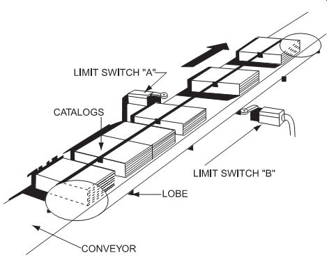
FIG. 1.1: Limit switches on a conveyor.

Limit switches contain a set of contacts. When a target object comes into contact with a limit switch's actuator on the conveyor in FIG. 1.1, the switch operates.

Various limit switches provide years of reliable operation even in the most demanding environmental conditions. They are appropriate for:

¦ Material handling

¦ Breweries

¦ Packaging machinery

¦ Wood products

¦ Special machinery

¦ Garbage compactors/trucks

¦ Valves

¦ Foundry equipment

Limit switches are available in explosion-proof versions to contain and cool escaping hot gases that otherwise could cause an explosion outside the switch in:

¦ Petroleum plants

¦ Chemical plants

¦ Waste treatment facilities

¦ Power generating stations

¦ Hazardous material handling

¦ Grain storage/handling

¦ Deep sea oil well platforms

Selecting and Specifying Limit Switches

Limit switches can be ordered with a variety of actuators, including plungers, rotary levers, and "wobble levers," which are flexible spring-like levers that operate by any movement except direct pulling.

FIG. 1.2 shows how characteristics are measured for rotary actuation, and FIG. 1.3 applies to limit switches actuated by in line plungers.

The characteristics of rotary-actuated limit switches are shown in degrees of angular rotation. The operating characteristic dimensions on enclosed switches for harsh environments are often shown in linear dimensions with the adjustable lever in one extreme position.

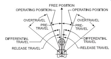
FIG. 1.2: Operating characteristics for rotary-actuated limit switches.

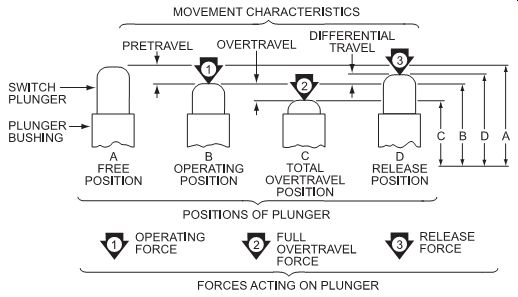
FIG. 1.3: Operating characteristics for limit switches with in-line plunger actuators.

Linear dimensions for in-line actuation are from the top of the plunger to a reference line, usually the center of the mounting holes. In the case of flange- or bottom-mounted switches, the reference line is the bottom of the switch.

To select the right limit switch for your application, consider:

¦ Actuator type

¦ Circuitry

¦ Ampere rating

¦ Supply voltage

¦ Housing material

¦ Termination type

Applicable Standards for Limit Switches

IEC (International Electrotechnical Commission), www.iec.ch/, especially JIC 60947-1 and IEC 60947-5-1, which explain the general rules relating to low-voltage switch and control gear for industrial use; IEC 529 rates the level of protection provided by enclosures, using an IP (International Protection) rating system.

CENELEC (The European Committee for Electrotechnical Standardization), www.cenelec.org, especially EN 50041 and EN 50047, which define characteristics and dimensions for limit switches.

NEMA (National Electrical Manufacturer's Association), www.nema.org. NEMA rates the protection level of enclosures as does IEC 529, but includes tests for environmental conditions, such as rust, oil, etc. that are not included in IEC 529.

Interfacing and Design Information for Limit Switches

Here are some considerations for incorporating limit switches in your designs.

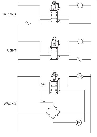
FIG. 1.4: Opposite polarities should not be connected to the contacts of one limit switch unless the switch is specifically designed for this.

FIG. 1.5: Power from different sources should not be connected to the contacts of one switch unless it is specifically designed for this.

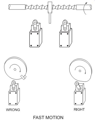
FIG. 1.6: Where relatively slow motion operates a limit switch, you'll generally want to apply a snap-action switch.

FIG. 1.7: Where relatively fast motion operates the switch, cams should be arranged so that the switch does not receive a severe impact.

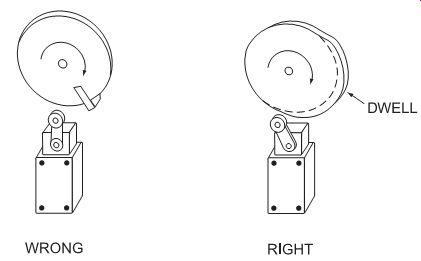
FIG. 1.8: Where relatively fast motions are involved, cams should be designed such that the limit switch will be operated long enough to operate relays, valves, etc. as needed.

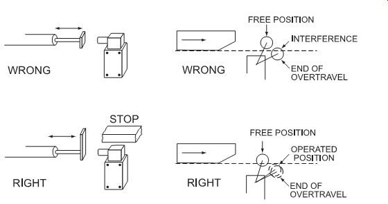
FIG. 1.9: Operating mechanisms for limit switches should be designed so that under any operating or emergency conditions, the switch is not operated beyond its overtravel limit position. A limit switch should not be used as a mechanical stop.

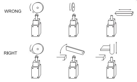
FIG. 1.10: For limit switches with pushrod actuators, the actuating force should be applied as nearly as possible in line with the pushrod axis. The same holds true for other actuators. For instance, the actuating force of a lever actuator should be applied as nearly perpendicular to the lever as practical and perpendicular to the shaft axis about which the lever rotates.

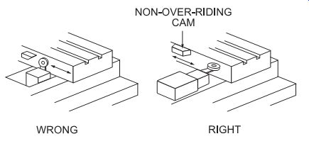
FIG. 1.11: Mount the switch rigidly in a readily accessible location. Cover plates should face the maintenance access point.

Resistive position sensors, also called potentiometers or simply position transducers, were originally developed for military applications. They were widely used as panel mounted adjustment knobs on radios and televisions in the years before pushbuttons and remote controls. Today, potentiometers are most commonly found in industrial applications that range from forklift throttles to machine slide sensing.

Potentiometers are passive devices, meaning they require no power supply or additional circuitry to perform their basic linear or rotary position sensing function. They are typically operated in one of two basic modes: rheostat and voltage divider (true potentiometric operation). As resistance varies with motion, rheostat applications make use of the varying resistance between a fixed terminal and the sliding contact wiper. In voltage divider applications, a reference voltage signal is applied across the resistive element track so that the voltage "picked up" by the movable contact wiper can be used to determine the wiper's position.

Advantages of potentiometers include low cost, simple operational and application theory, inherent absolute measurement even through power-off cycles, and robust EMI emission/susceptibility performance. Disadvantages include eventual wear-out due to the sliding contact wiper and sensing angles that are limited to less than 360 degrees, although vernier drives can be applied to give them "multi-turn" sensing capability.

Selecting and Specifying Resistive Position Sensors

For many general-purpose position sensing applications, a low-cost potentiometer is often more than adequate. In some cases (certain electric motor controllers, for example), a changing resistance is expected as the control signal, and thus a potentiometer is really the only choice. In most other applications, a fixed reference voltage is applied, and a voltage reading at the wiper terminal senses the position. Rotary potentiometers can offer linearity errors on the order of 1% maximum and rotational lifetimes of a million or more cycles. For more critical applications, higher-precision potentiometers can offer linearity errors a hundred or more times better than this, and rotational lifetime ratings in the tens or even hundreds of million cycles.

In looking for the best cost versus performance trade-off, consider the system as well as the transducer. Usually you will take one of two paths to select a transducer:

¦ Find a transducer that works with the power supplies and amplifiers or controllers in your system.

¦ Select the position transducer and then match your system components to it.

What is the length to be measured?

For potentiometers this is called the theoretical electrical travel. For most applications this is straightforward; however, there are times where you may want to measure only a portion of the total travel of your system. For example, it may be advantageous to have the highest possible resolution at one end of the system's travel. Consider a 10-inch total travel, but by monitoring the last inch, you can increase your resolution tenfold.

What accuracy can I get?

Accuracy can have several meanings. Do you mean how small a motion you can pick up (resolution)? How much error there is at any point along the electrical travel compared to a reference line (independent linearity)? Is the output the same at a given point from one cycle to another (repeatability)? These are not the same, but any one is often called ''accuracy." It is important to differentiate and prioritize these performance parameters. Many conductive plastic position transducers have infinite resolution. The repeatability with most transducers is excellent and will rarely be more than the signal-to-noise ratio that will likely exist in your system. Look for independent linearity, the error versus the reference line, guaranteed to be less than 0.1%.

How rugged does the transducer need to be? The unit's ability to hold up under high levels of shock, vibration, moisture, dirt, oil or temperature extremes is sometimes more important than accuracy. What good is a high-accuracy device if it won't last long in the application? Conductive plastic with stands many harsh chemicals and will work immersed in hydraulic oil.

What excitation should I use? For potentiometers, the excitation is determined by the input of your signal conditioner or the controller you are using. You will need to decide whether to use regulated or unregulated voltage, depending on your conditioner or controller.

What mounting factors should I consider?

These vary from application to application. Proper alignment of the shaft of the potentiometer is important for maximum life from the unit. Mounting should allow for minor adjustment to minimize any misalignment. Rod ends or shaft couplings are an effective way to compensate for misalignment. Side load on a potentiometer will wear out the bearings long before the wiper or element fail, so careful mounting is to your advantage. If there is heavy hose down or spray from oil or water, you should use a water-resistant or waterproof potentiometer.

Does the transducer need to be compensated for temperature effects?

Potentiometers, while they have measurable temperature coefficients, will not usually require temperature compensation because they are most often used as voltage dividers.

Applicable Standards for Resistive Position Sensors

The Variable Electronics Component Institute (http://www.veci-vrci.com) has developed a number of testing and performance standards governing potentiometers.

While their standards are not binding on manufacturers, they help ensure practical, meaningful and consistent terminology and methodologies. Many potentiometers also conform to military standards such as MIL-STD-202F.

Interfacing and Design Information for Resistive Position Sensors

For the most part, using a resistive position sensor is quite straightforward. First, establish what sort of electrical signal is needed from the mechanism being sensed.

If a resistance change is needed, connect one end of the potentiometer and the wiper terminal into the circuit. Resistance will then vary with motion in this mode (rheostat mode); contact noise (an unpredictably varying resistance) will appear superimposed on the expected smooth change of resistance. Contact noise results from the variation in mechanical contact between the wiper and the resistive element's surface. It manifests as a series resistance between the element surface (contact point) and the wiper terminal. It can vary from a fraction of a percent up to 5% or more of the total element resistance.

Voltage divider mode operation is by far more prevalent in position sensing applications, and in this mode, the effects of contact resistance variation are diminished or eliminated. Its output is a voltage ratio determined from the wiper voltage divided by the applied voltage. The output voltage is taken from the wiper terminal. Thus, if little or no current is flowing through this path (as is the case when the voltage feeds a high-impedance measurement circuit), the series contact resistance variation creates no change in the voltage between the contact point and the wiper terminal.

When an excitation voltage is applied across the resistive element, the wiper moves from the zero voltage end of the element toward the maximum output end. The voltage between the wiper and the resistive element varies linearly with position. (See FIG. 1.12.) The maximum output voltage of the sensor never exceeds the applied voltage.

For example, if you apply 10 volts to the resistive element, the maximum output voltage is 10 volts. The wiper will vary from 0 to 10 volts, with 5 volts at the center position. If you apply 5 volts, an output of 2.5 volts indicates the center position.

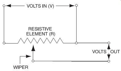
FIG. 1.12: Potentiometer component.

Magnetic Position Sensors

Magnetic properties can be used to determine position by detecting the presence, strength, or direction of magnetic fields not only from the Earth but also from magnets, fields generated from electric currents, and even brain wave activity. Magnetic sensors can measure these properties without physical contact and have become the eyes of many industrial and navigation control systems.

The magnetic field is a vector quantity that has both magnitude and direction. Magnetic sensors measure this quantity in various ways. Some magnetometers measure total magnitude but not direction of the field (scalar sensors). Others measure the magnitude of the component of magnetization along their sensitive axis (uni-directional sensors). This measurement may also include direction (bi-directional sensors). Vector magnetic sensors have two or three bi-directional sensors. Some magnetic sensors have a built-in threshold and produce an output only when that threshold is passed.

A Hall effect device derives its output from magnetic field strength, while a magneto resistive device measures the angle direction of a magnetic field, so its output is based on the electrical resistance of the field. Some of the advantages of measuring field direction vs. field strength include:

¦ Insensitivity to the temperature coefficient of the magnet,

¦ Less sensitivity to shock and vibration, and

¦ The ability to withstand large variations in the gap between the sensor and the magnet.

Hall effect position sensors are very affordable and accurate. They contain a Hall element constructed from a thin sheet of conductive material with output connections perpendicular to the direction of current flow. When subjected to a magnetic field, a Hall sensor responds with an output voltage proportional to the strength of the field.

The voltage output is very small and requires additional electronics to achieve useful voltage levels. These signal-conditioning electronics are combined with a Hall element on an integrated circuit (IC) to form a basic Hall effect sensor.

Magneto-resistive (MR) sensors are usually made of a nickel-iron (Permalloy) thin film deposited on a silicon wafer and patterned as a resistive strip. The properties of the MR thin film cause it to change resistance by 2 to 3% in the presence of a magnetic field. For a typical MR sensor, the bandwidth is in the 1 to 5 MHz range. Reaction is very fast and not limited by coils or oscillating frequencies.

MR sensors measure both linear and angular position and displacement in the Earth's magnetic field (below 1 gauss). They are an excellent solution for locating objects in motion. By affixing a magnet or sensor element to an angular or linear moving object with its complementary sensor or magnet stationary, the relative direction of the resulting magnetic field can be quantified electronically.

The demand for Hall effect magnetic sensors remains high because the Hall effect is the only magnetic effect that can be implemented in a standard complementary metal oxide semiconductor (CMOS) technology, which makes them very affordable. Some of the advantages of Hall effect sensing devices include their long life and high speed.

They operate with stationary input (zero speed), and have a broad temperature range (-40 to +150 degrees C) for industrial and automotive applications.

While Hall effect is highly linear with no saturation effects out to extremely high fields, magneto-resistance is roughly 200 times more sensitive than the Hall effect in silicon, so it can be used for longer sensor-to-magnet distances.

A unique aspect of using magnetic sensors is that measuring magnetic fields is usually not the primary intent. Another parameter, such as wheel speed or the position of a part, is sought. Magnetic sensors don't measure these parameters directly but extract them from changes in magnetic fields.

The enacting input has to create or modify a magnetic field. Once the sensor detects the field or change to a field, the output signal requires some signal processing to translate the sensor output into the desired parameter value. This makes magnetic sensing a little more difficult to apply in most applications, but it also allows for reliable and accurate sensing of parameters that are difficult to sense otherwise.

Selecting and Specifying Magneto-resistive Position Sensors

MR sensors can detect the presence of a vehicle from a distance of about 50 feet and are often used in traffic and toll way applications. Other common applications include automotive wheel speed, crankshaft sensing and compass navigation. An area of growth for MR sensors is high-density read heads for tape and disk drives. MR sensors are beneficial in applications for linear position or linear displacement, LVDT (linear variable differential transformer) replacements, proximity detection, valve positioning, shaft travel, automotive steering, robotics, brake and throttle position systems. By utilizing an array of magnetic sensors or magnets, the capability of extended range angular or linear position measurements can be achieved.

MR sensors come in a variety of shapes and forms and can sense DC static fields as well as the strength and direction of the field. The long span absolute linear position (Honeywell patented) sensing solution illustrated in FIG. 1.13 utilizes an array of MR sensors, a magnet and signal conditioning electronics. The sensors are used to determine the position of a magnet that is attached to a moving object. In addition to the mechanical benefits of no moving parts to wear out and no dropped signals from worn tracks, this solid state solution provides high accuracy with low power and works in rugged environments, such as high temperature.

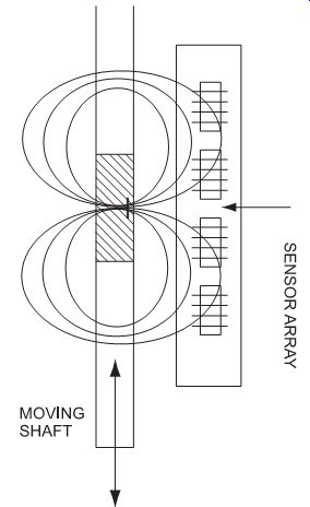
FIG. 1.13: System design with an array of four magneto-resistive sensors.

This array device is designed to be sensitive to the direction of a magnetic field when it operates in saturation mode. The saturation mode is when external magnetic fields are above a certain field strength level (called saturation field). The magnetic moments in the device are aligned in the same direction of the field. Therefore, the output of the de- vice only reflects the direction of the external magnetic field and not its strength. The incentive of operating in saturation mode includes:

¦ Immunity to temperature coefficient of magnet,

¦ Insensitivity to the gap between the magnet and the sensor array, and

¦ Insensitivity to magnetic field strength when the field is greater than saturation level.

The saturation field of this type of sensor is 30-50 gauss. Magnetic fields in this magnitude can be easily provided by any permanent magnet, including low cost AlNiCo or ceramic magnets, unlike Hall effect devices that require a stronger magnet.

Magneto-resistive sensors bring a unique feature to this solution by measuring the angle direction of a field from a magnet versus the strength of a magnetic field. A permanent magnet provides the magnetic field, which has the function of keeping the sensors in saturation mode, minimizing effects of stray magnetic fields and providing a linear operating range for selected sensor pairs.

Unlike other incremental sensors, this technology is absolute reading; no reference point is required. Position is accurately known at any time as well as at power-on.

When each sensor in the array is connected to the supply voltage, it converts any ambient, or applied magnetic field to a voltage output.

MR sensors provide highly predictable outputs. Their high sensitivity, small size, noise immunity, and reliability are advantages over mechanical or other electrical alternatives.

Highly adaptable and easy to assemble, these sensors solve a variety of problems in custom applications. One of the key benefits of MR sensors is that they can be bulk manufactured on silicon wafers and mounted in commercial integrated circuit packages. This allows magnetic sensors to be auto-assembled with other circuit and systems components.

Selecting and Specifying Hall Effect Position Sensors

Hall sensors find a wide variety of position applications, especially as proximity sensors. They are used extensively in automobiles to sense everything from the positions of pistons and the angles of throttles, to power window and door interlock positions.

They show up in office machines where they sense things like paper placement and in cameras to detect shutter position. On factory floors they are used to control every thing from motor speeds to drilling machines.

Both digital and analog Hall effect position sensors are available. Digital output sensors are in one of two states: ON or OFF. Analog sensors provide a continuous voltage output that increases with a strong magnetic field and decreases with a weak magnetic field. Both are operated by the magnetic field from a permanent magnet or an electromagnet with actuation mode, depending on the type of magnets used.

There are two types of digital sensors: bipolar and unipolar. Bipolar sensors require positive gauss (south pole) to operate and negative gauss (north pole) to release. Uni polar sensors require a single magnetic pole (south) to operate. Release is obtained by

[...]

Vector Hall sensors have four Hall elements on a single die (two for the X axis and two for the Y axis) to provide a differential output voltage for each axis. The signal pair is "gain matched" so that the mathematical ratio of the two signals cancels out any variation in gain or field strength due to temperature or a mechanical shift, such as shock or vibration. This not only reduces offset but also allows for relatively wide tolerance of axial and radial misalignment of the magnet and sensor, making the installation process less critical. The time required for the microprocessor to process this ratio determines the maximum rate of position updates and does limit the usable rotational speed of the sensor somewhat.

Some manufacturers offer automatic indexing to set a mechanical "zero" or "index" position whenever a particular signal is applied to the circuit. For example, this can be accomplished by shorting the output to I-V while bringing up the power. An indexing feature eliminates significant rigging and alignment at installation.

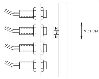
FIG. 1.15: Four digital output, bipolar sensors are actuated by one magnet mounted on a rod.

Interfacing and Design Information for Magnetic Position Sensors

Begin your design by determining sensing specifications. For sensing systems actuated by a magnet, specifications include:

¦ The minimum and maximum gap between the magnet and the position sensor,

¦ The limits of magnet travel,

¦ Special requirements for the magnet such as high coercive force due to ad verse magnetic fields in the system,

¦ Mechanical linkages (if required),

¦ Sensor output type (NPN or PNP),

¦ Operating temperature range,

¦ Storage temperature range, and

¦ Various input/output specifications from the system specification.

The next step is to choose the magnetic mode, magnet, sensor, and functional inter face. These four items are interdependent. The required magnet strength is dependent on the gap and the limits of magnet travel (magnetic mode). The sensor is dependent on the strength of the magnetic field and therefore, on the magnetic mode and the magnet chosen. The functional interface is dependent on the sensor output type and electrical characteristics.

Figs 1.16-20 illustrate a few of the ways a magnetic system can be presented to a linear output sensor for position measurement as listed in the comparison chart. The method of actuation is determined based upon cost, performance, accuracy and other requirements for a given application.

A simple method of position sensing is shown in FIG. 1.16. One pole of a mag net is moved directly to or away from the sensor. This is a unipolar head-on position sensor. When the magnet is farthest away from the sensor, the magnetic field at the sensing face is near zero gauss. In this condition, the sensor's nominal output voltage will be 6 volts with a 12-volt supply. As the south pole of the magnet approaches the sensor, the magnetic field at the sensing surface becomes more and more positive. The output voltage will increase linearly with the magnetic field until a +400 gauss level or nominal output of 9 volts is reached. The output as a function of distance is nonlinear, but over a small range may be considered linear.

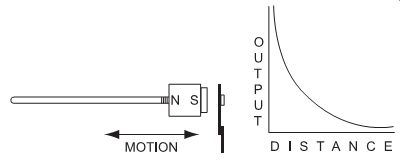
FIG. 1.16: Unipolar head-on position sensor.

Bipolar head-on sensing is shown in FIG. 1.17. When the magnets are moved to the extreme left, the sensor is subjected to a strong negative magnetic field by mag net #2, forcing the output of the sensor to a nominal 3.0 volts. As magnet #1 moves toward the sensor, the magnetic field becomes less negative until the fields of magnet #1 and magnet #2 cancel each other (at the midpoint between the two magnets). The sensor output will be a nominal 6.0 volts. As magnet #1 continues toward the sensor, the field will become more and more positive until the sensor output reaches 9.0 volts.

This approach offers high accuracy and good resolution as the full span of the sensor is utilized. The output from this sensor is linear over a range centered on the null point.

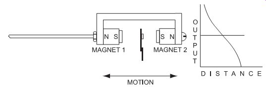
FIG. 1.17: Bipolar head-on position sensor.

Biased head-on sensing, a modified form of bipolar sensing, is shown in FIG. 1.18. When the moveable magnet is fully retracted, the sensor is subjected to a negative magnetic field by the fixed bias magnet. As the moveable magnet approaches the sensor, the fields of the two magnets combine. When the moveable magnet is close enough to the sensor, it will "see" a strong positive field. This approach features mechanical simplicity.

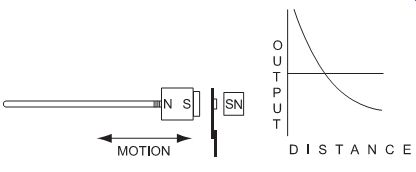
FIG. 1.18: Biased head on position sensor.

Slide-by actuation is shown in FIG. 1.19. A tightly controlled gap is maintained between the magnet and the sensor. As the magnet moves back and forth at that fixed gap, the field seen by the sensor becomes negative as it approaches the north pole, and positive as it approaches the south pole. This type of position sensor features mechanical simplicity, and when used with a long enough magnet, can detect position over a long magnet travel. The output characteristic of a bipolar slide-by configuration is the most linear of all systems illustrated, especially when used with a pole piece at each pole face. However, tight control must be maintained over both vertical position and gap to take advantage of this system's characteristics.

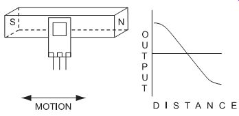
FIG. 1.19: Slide-by position sensor.

Some descriptive terms:

Motion type refers to the manner in which the system magnet may move. These types include:

¦ Continuous motion (motion with no changes in direction),

¦ Reciprocating motion (motion with direction reversal), and

¦ Rotational motion (circular motion that is either continuous or reciprocating).

Mechanical complexity refers to the level of difficulty in mounting the magnet(s) and generating the required motion.

Symmetry refers to whether or not the magnetic curve can be approached from either direction without affecting operate distance.

Digital refers to the type of sensor, either unipolar or bipolar, recommended for use with the particular mode.

Linear refers to whether or not a portion of the gauss versus distance curve (angle relationship) can be accurately approximated by a straight line.

Precision refers to the sensitivity of a particular magnetic system to changes in the position of the magnet.

A definite relationship exists between the shape of a magnetic curve and the precision that can be achieved. Assume the sloping lines in FIG. 1.20 are portions of two different magnet curves; 01 and 02 represent the range of actuation levels (unit to unit) for digital output Hall effect sensors. It is evident from this illustration that the curve with the steep slope (B) will give the smaller change in operate distance for a given range of actuation levels.

Thus, the steeper the slope of a magnetic curve, the greater the accuracy that can be achieved.

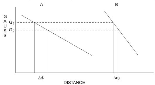
FIG. 1.20: Effect of slope

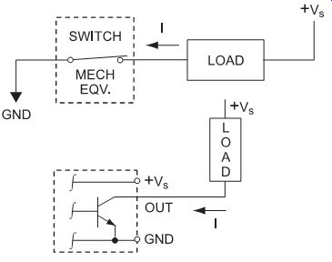
FIG. 1.21: Typical digital Hall effect NPN output.

FIG. 1.21 shows the output of a digital Hall effect sensor. The sensor in this particular example is NPN (current sinking, so the current flows from the load into the sensor, open collector) in the actuated (ON) state. Current sinking devices contain NPN integrated circuit chips. Like a mechanical switch, the digital sensor allows current to flow when turned ON, and blocks current flow when turned OFF. Unlike an ideal switch, a solid state sensor has a voltage drop when turned ON, and a small current (leakage) when turned OFF. The sensor will only switch low-level DC voltage (30 VDC max.) at currents of 20 mA or less. In some applications, an output interface may be current sinking output.

FIG. 1.22 illustrates supply for an NPN (current sinking) sensor. In this circuit configuration, the load is generally connected between the supply voltage and the out put terminal (collector) of the sensor.

When the sensor is actuated, turned ON by a magnetic field, current flows through the load into the output transistor to ground.

The sensor's output voltage is measured between the output terminal (collector) and ground (-). When the sensor is not actuated, current will not flow through the output transistor (except for the small leakage current).

The output voltage, in this condition, will be equal to VLS (neglecting the leakage current). When the sensor is actuated, the output voltage will drop to ground potential if the saturation voltage transistor is neglected. In terms of the output voltage, an NPN sensor in the OFF condition is considered to be normally high.

There are several methods for linearizing output for analog magnet sensors. The output of the sensor as a function of magnetic field is linear, while the output as a function of distance may be quite nonlinear.

Sensor output can be converted to one that compensates for the non-linearities of magnetics as a function of distance. One method involves converting the analog output of the sensor to digital form. The digital data is fed to a microprocessor, which linearizes the output through a ROM look-up table or transfer function computation techniques (FIG. 1.23).

A second method involves implementing an analog circuit that has the necessary transfer function to linearize the sensor's output (FIG. 1.24).

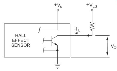
FIG. 1.22: The supply voltage (Vs) need not be the same as the load supply (VLS); however, a single supply is usually convenient.

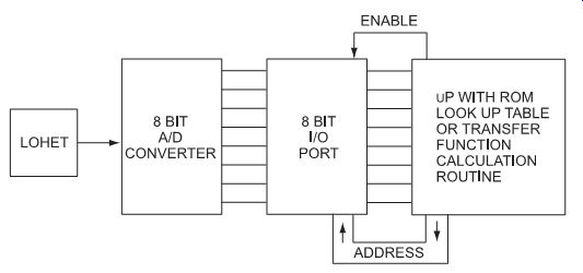
FIG. 1.23: Microprocessor linearization.

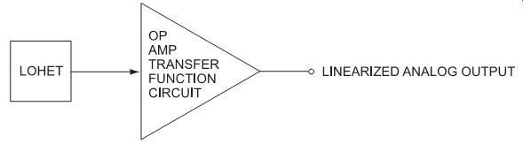
FIG. 1.24: Analog linearization

A third method for linearizing the sensor output can be realized through magnetic design by altering the geometry and position of the magnets used. These types of magnetic assemblies are not normally designed using theoretical approaches. In most instances, it is easier to design magnetics empirically by measuring the magnetic curve of the particular assembly. By substituting a calibrated Hall element for the variety of magnetic systems available, the designer can develop systems that perform a wide variety of sensing functions.

Ultrasonic Position Sensors

Ultrasonic sensors provide precise no-touch presence/absence sensing and distance sensing or tracking. They are particularly useful where other sensing technologies have difficulty, such as with clear or shiny target objects, foggy or particle-laden air, and environments with splashing liquids. Ultrasonic solutions are often used where larger sensors or longer sensing distances are required.

Factory noise does not affect ultrasonic sensor operation because their operating frequency is well above the frequency of ambient sound. And because sound is used, air pressure, humidity, and smoke, dust, vapors and other airborne contaminants have little effect on accuracy. They provide an alternative to photoelectric or proximity sensors in applications where target characteristics or environmental factors interfere with performance, such as:

¦ Material handling,

¦ Packaging,

¦ Paper processing,

¦ Food and beverage,

¦ Chemical,

¦ Plastics industry, Rubber/tire processing, and

¦ Steel processing.

Ultrasonic sensors work by exciting an acoustic transducer with voltage pulses, causing the transducer to vibrate ultrasonically. These oscillations are directed at a target and, by measuring the time for the echo to return to the transducer, the target's distance is calculated. Ultrasonic sensors generally provide an accuracy of 1 mm at distances ranging from 100 mm to 6,000 mm (over 19 feet).

Ultrasonic sensors have no difficulty working with round, moving targets, such as film, paper, rubber or steel. (See FIG. 1.25.) Ultrasonic sensors often are used for fill-level control for both solids and liquids in the food and beverage, chemical and plastics industries. They can detect the presence of glass parts and provide a simple but highly effective warning system to prevent dam age in warehouses when a forklift or other vehicle is in danger of a collision.

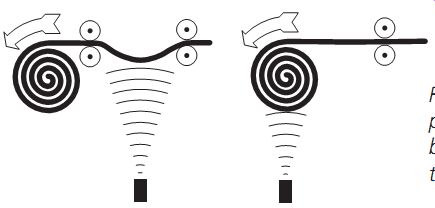
FIG. 1.25: Two ultrasonic sensors provide roll diameter and tension control by providing outputs directly proportional to distance and roll diameter.

Selecting and Specifying Ultrasonic Sensors

Since ultrasonic sensors operate on an elapsed time measurement system, when the sensor is adjusted to sense a target at a given distance, a timing window is established.

The sensor accepts or acknowledges only the echoes received within this window.

Signals echoing from background material take longer and will not be acknowledged.

The maximum switching frequency is the rate at which the sensor is capable of turning on and off. It depends on several variables. The most significant are target size, target material and distance to the target. The smaller the target, the more difficult it is to detect. Thus, maximum frequency for a small target will be lower than for a large target. Materials that absorb high frequency sound (cotton, sponge, etc.) are more difficult to sense than steel, glass, or plastic. Thus, they also have a lower maximum switching frequency.

Target-to-sensor distance is very important in determining maximum switching frequency. The sensor sends an ultrasonic beam though the air. It takes a finite time for the signal to leave the sensor, travel to the target, strike the target, and return to the sensor as an echo. The farther a target is from the sensor, the longer it takes the sound to complete this cycle, and the lower the switching frequency.

Surface finish is also a consideration. If a smooth flat target is inclined more than +3 degrees to the normal of the beam axis, part of the signal is deflected away from the sensor and the sensing distance is decreased. However, for small targets located close to the sensor, the deviation from normal may be increased to +8 degrees. If the target is inclined more than approximately 12 degrees to the normal of the beam axis, the entire signal is deflected away from the sensor, and the sensor will not respond. A beam striking a target with a coarse surface (such as granular material) is diffused and reflected in all directions and some of the energy returns to the sensor as a weakened echo. (See FIG. 1.26.)

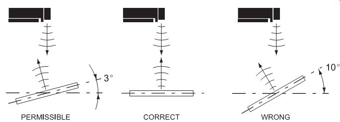
FIG. 1.26: Maximum inclination for smooth, flat targets.

The velocity of sound in air is temperature dependent. An internal temperature sensor adapts the clock frequency of the elapsed time counter and carrier frequency to help compensate for variations in air temperature. However, larger temperature fluctuations within the beam path can cause dispersion and refraction of the ultrasonic signal, adversely affecting the measurement accuracy and stability (FIG. 1.27). If a hot object must be detected, experiment by positioning the sensor and target on a vertical plane and aim at the lower (cooler) portion of the target. In this way, it may be possible to avoid the warm air currents and achieve satisfactory operation.

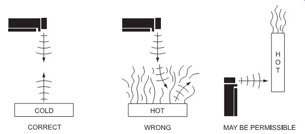
FIG. 1.27: Sound dispersion due to warm air currents.

Ultrasonic sensors have a "dead zone" in which they cannot accurately detect the target (FIG. 1.28). This is the distance between the sensing face and the minimum sensing range. If the target is too close, the tone burst's leading edge can travel to the target and strike it before the trailing edge has left the transducer. Echo information returning to the sensor is ignored because the transducer is still transmitting and not yet receiving. The echo generated could also reflect off the face of the sensor and again travel out to the target. These multiple echoes can cause errors when the target is in the dead zone.

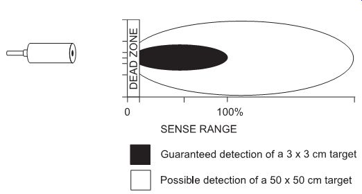
FIG. 1.28: Ultrasonic sensors must be mounted outside of the dead zone.

Maximum sensing distance or range for each target and application is determined experimentally. Figures 1.29-31 show sensitivity characteristics and typical sensing distances.

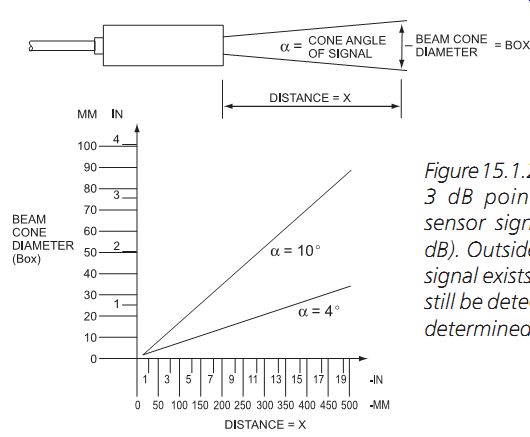
FIG. 1.29: Beam cone angle values are the 3 dB points (i.e., points at which the sensor signal is attenuated by at least 3 dB). Outside this cone angle, the ultrasonic signal exists but is rather weak. Targets may still be detected. This can be experimentally determined.

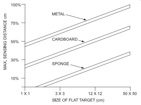
FIG. 1.30: Sensing range with maximum sensitivity.

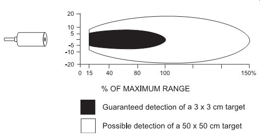
FIG. 1.31: Target size versus beam spot.

The ultrasonic sensor emits a sound beam in a beam cone angle that eliminates side lobes. Target size versus beam spot size is important. Theoretically, the smallest detectable target is one half the wavelength of the ultrasonic signal. At 215 kHz, the signal wavelength is 0.063 in. Under ideal conditions, these sensors are capable of sensing targets as small as 0.032in. Targets usually are larger and are sensed at various distances. In order to estimate the area covered by the ultrasonic signal at a given distance, use the formula: Box - 2 × 1 tan (K/2)

Where:

Box = Beam Cone Diameter at distance

X = Distance, target to sensor

K = Beam Cone Angle

The beam cone angle can be halved using a beam cone concentrator.

Normal atmospheric air pressure changes have no substantial effect on measurement accuracy. Ultrasonic sensors are not intended for use in areas with high or low air pressure changes.

The effect of humidity on measurement is virtually negligible, amounting to only 0.07% for a change of relative humidity of 20%. Absorption of sound increases, how ever, with increasing humidity. Thus, the maximum measurement distance is slightly reduced.

Air turbulence, air currents and layers of different densities cause refraction of the sound wave. An echo may be produced, and the signal weakened or diverted to the extent that the echo is not received. Maximum sensing range, measurement accuracy and measurement stability can deteriorate under these conditions.

Protective measures for the sensor may include a silicone rubber coating when a device is used in an aggressive acid or alkaline atmosphere. To maintain operating efficiency, care must be taken to prevent solid or liquid deposits of these potentially destructive materials from forming on the sensor face.

Interfacing and Design Information for Ultrasonic Sensors

A feature to consider in your design includes an inhibit/sync signal setting. This disables the transmitter, preventing it from sending out any signals. This signal can be used to multiplex/synchronize two or more sensors that are mounted close to each other where acoustic interference is possible. Inhibit multiplexes the sensors so that only one transmits the ultrasonic signal at a given time. Also, the inhibit signal wires from all the sensors can be connected together, synchronizing the sensors to transmit at the same time.

In reflective applications, optional beam deflectors can be used to deflect the beam 90 degrees, helping to reduce the space required for mounting the sensors. Beam concentrators reduce the beam diameter approximately one half. This improves accuracy when measuring liquids, while extending the sensing range as much as 125%. Concentrators are also helpful when sensing small parts.

Proximity Sensors

Proximity sensors are low cost, solid-state devices that come in a variety of technologies, configurations and sensing ranges. They feature fast operation, choice of AC or DC, inherent long life, and compatibility with industrial controllers.

Inductive proximity sensors detect all metals, ferrous metals only, or non-ferrous metals only. Capacitive sensors detect all materials.

FIG. 1.32: Proximity sensors detect bottle caps.

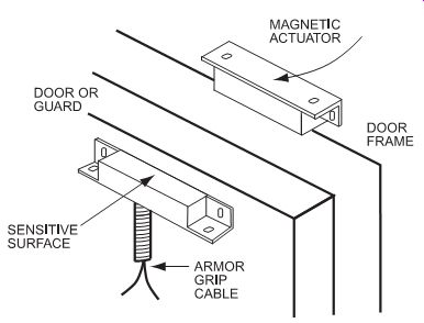
FIG. 1.33: A proximity sensor acts as a door guard.

Capacitive proximity sensors have an oscillating electric field, sensitive to all materials: dielectric materials, such as glass, rubber and oil; and conductive materials, such as metals, salty fluids and moist wood. Capacitance (C) is a function of the size of the electrodes (A), the distance between them (d), and the dielectric constant (D) of the material between the electrodes (air =1.0). See FIG. 1.34.

Capacitance = C D A d

FIG. 1.35 illustrates a simple capacitive sensor. The top electrode is the face of the sensor. A seal ring, the target, passes between it and the ground electrode (a metal conveyor belt). The sensor housing insulates the electrode from galvanic coupling to ground. The rubber seal ring has a dielectric constant (D) of 4.0. When it enters the electric field, the capacitance increases. The sensor detects the change in capacitance and provides an output signal.

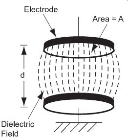
FIG. 1.34: The oscillating electric field of a capacitive proximity sensor responds to the dialect constant of the target.

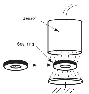
FIG. 1.35: A capacitive proximity sensor detects a change in capacitance incurred by the presence of a seal ring target.

FIG. 1.36 illustrates a metal target, or some other conductive material, entering the electric field. The resulting increase in capacitance is detected and converted to an output signal.

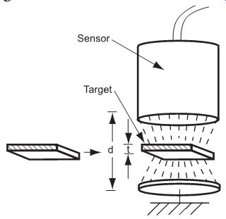
FIG. 1.36: Presence of the metal target reduces the effective distance between electrodes (by the factor t), resulting in an increase in capacitance.

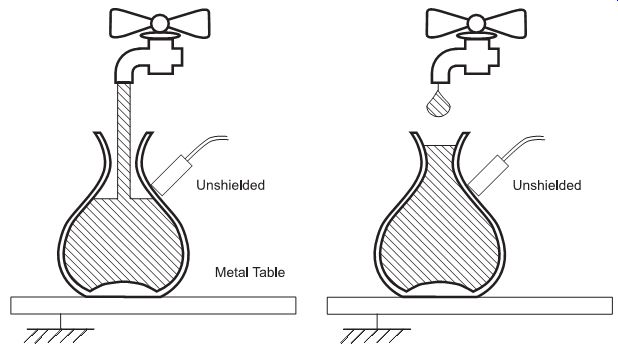
FIG. 1.37: Once the ground electrode provided by the fluid is in place, the circuit closes and a signal results.

The level of conductive fluid pouring into a glass bottle is below the sensor (FIG. 1.37). With no change in capacitance, there is no output. Once the fluid has reached the level of the sensor, it provides the ground electrode. This happens even though the glass of the bottle separates the fluid and the metal table. The three materials form a capacitor. The alternating current provides a path to ground.

FIG. 1.38 shows an unshielded sensor and a shielded sensor working together.

The shielded sensor locates the glass bottle so it can be filled with liquid. The un shielded sensor indicates that the fill level is reached and it can be turned off. Note that shielded sensors may be flush mounted in any solid material.

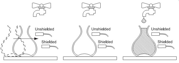
FIG. 1.38: Neither sensor switches as the bottle approaches. Once the shielded sensor detects the entrance of the glass into its electric field, it switches.

When the fluid reaches the level of the unshielded sensor, it switches.

Without some sort of compensation, any material entering the sensing field can cause an output signal. This includes water droplets on the sensor face, dirt or dust, and other contaminants. A compensation electrode in the sensor solves this problem by creating a compensation field.

(See FIG. 1.39.) When contaminants lie directly on the sensor face, both fields are affected, and the capacitance increases by the same ratio. The sensor does not see this as a change in capacitance, and an output is not produced.

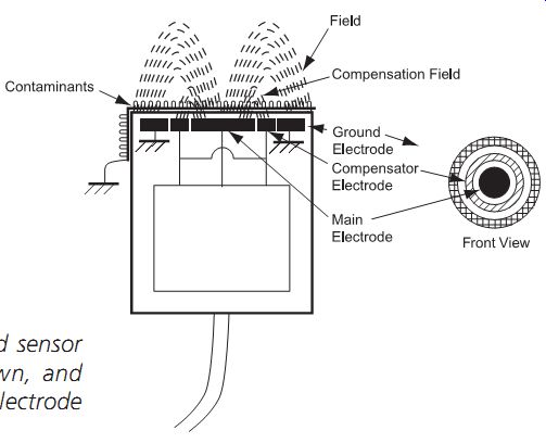
FIG. 1.39: Shows a shielded sensor with two sensing fields-its own, and the compensation field that the electrode created.

Sr = Sn ± (.10 × Sn)

Temperature drift tolerances must be also calculated. Over a range of -25 to +70°C, a sensing distance drift of +10% can be expected. Over -25 to +85°C, the tolerance increases to +15%.

Su = Sr ± (.10 × Sr) -25 to +70°C

Su = Sr ± (.15 × Sr) -25 to +85°C

Usable sensing distance (Su) of any sensor can now be estimated. Su is the distance at which the sensor will always operate. If the target-to-sensor range is greater, the sensor may or may not operate reliably. (See FIG. 1.41.)

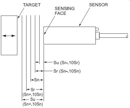
FIG. 1.41: Nominal sensing distance (Sn) versus usable sensing distance (Su).

Once the usable sensing distance is determined, you need to figure in the actual application conditions. There are three factors to take into account:

¦ Target material,

¦ Target size, and

¦ Target presentation mode.

The nominal sensing distance given in inductive proximity sensor specifications is determined with a target made of mild steel (in accordance with EN 60947-5-2). Whenever a target is a different metal, a correction needs to be made to the usable sensing distance (Su). The formula is:

New Su = Old Su × M

M = material correction factor

The standard target is a square of steel, 1mm (.04 in.) thick, with sides equal to sensor diameter. To determine the sensing distances for materials other than standard, a corresponding correction factor is used. Some common materials and their correction factors are listed in Table 1.1.

Table 1.1: Correction factors for non-standard target materials.

Mild steel targets of "standard" sizes are used to establish published sensing distances. The standard size for each size and style of sensor usually is given in the manufacturer's order guides. If your desired target is the same size or larger than the standard target, no correction factor is necessary. However, a smaller target affects sensing distance. The surface area of the application target versus the surface area of the standard target provides the correction factor. (See Table 1.2.) The formula is:

New Su = Old Su × T

T = target correction factor

Table 1.2: Correction factors for non-standard target sizes

When working with capacitive sensors, the dielectric constant of the target must be determined. All materials have a dielectric constant. This constant is what increases the capacitance level of the sensor to a set trigger point. The larger the dielectric constant, the easier a material will be to detect. Materials with high dielectric constants can be detected at greater distances than those with low constants. This allows materials with high dielectric constant to be sensed through the walls of containers made of a material with a lower constant. An example is the detection of salt (6) through a glass wall (3.7).

Each application should be tested. The list of dielectric constants in Table 1.3 is provided to help determine the feasibility of the application.

Table 1.3: Dielectric constants for different targets.

As shown in FIG. 1.42, there are two target presentation modes. Published sensing distances usually are determined by using the head-on mode of actuation.

The target can also approach the sensor in the slide-by mode. However, the slide-by method reduces actual sensor-to-target distance by 20%.

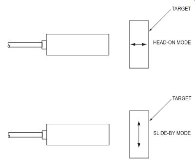
FIG. 1.42: Targets may be presented in head-on or slide-by mode.

Inductive proximity switches are available with a choice of switching functions. Normally open circuitry causes output current to flow when a target is detected; normally closed circuitry produces zero output current when a target is detected. Changeover circuitry has two sensing outputs; one conducts when a target is detected while the other will not.

Applicable Standards for Proximity Sensors

CENELEC (The European Committee for Electrotechnical Standardization), www.cenelec.org.

IEC (International Electrotechnical Commission), www.iec.ch/, especially IEC 60947-1 and IFC 60947-5-1, which explain the general rules relating to low-voltage switch and control gear for industrial use; IEC 529 rates the level of protection pro vided by enclosures, using an IP (International Protection) rating system.

Description of protective classes (EN 60529) common to proximity sensors:

¦ IP 65: Protection against ingress of dust and liquid

¦ IP 67: Protection against limited immersion in water and dust ingress under predetermined pressure and time conditions (1 meter of water for 30 minutes minimum)

¦ IP 68: Protection against the effects of continuous immersion in water NEMA (National Electrical Manufacturer's Association), www.nema.org. NEMA rates the protection level of enclosures as does IEC 529, but includes tests for environmental conditions, such as rust, oil, etc. that are not included in IEC 529.

UL (Underwriters Laboratories), www.ul.com.

Interfacing and Design Information for Proximity Sensors

When applying capacitive sensors, it's important to note that while shielded capacitive sensors may be flush-mounted, unshielded sensors require isolation-a material-free zone around the sensing face. Materials immediately opposite both shielded and un shielded sensors must be removed to avoid false actuation. See FIG. 1.43.

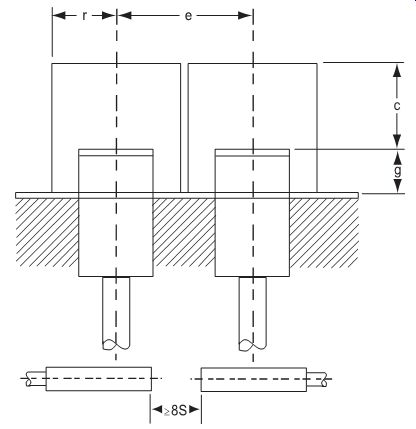
FIG. 1.43: Unshielded proximity sensors require isolation.

Device-to-device isolation is used when two or more sensors are mounted near each other to prevent cross talk and interference between the devices. Mounting distance between shielded capacitive proximity sensors (center to center) should be at least the diameter of the sensing face. Distance between unshielded sensors will vary and be three to four times the nominal sensing distance.

When shielded or unshielded sensors are facing each other, distance between sensing faces should be at least eight times the sensing distance. To ensure that both shielded and unshielded proximity switches function properly, and to eliminate the possibility of false signals from nearby metal objects, plan for minimum distances as shown in FIG. 1.44.

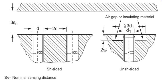
FIG. 1.44: Minimum distances for proximity sensors.

For unshielded proximity switches mounted opposite to each other or side by side, the minimum allowable distances in FIG. 1.45 apply:

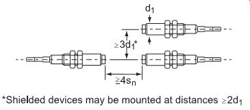
FIG. 1.45: Minimum mounting distances for unshielded sensors

The switching hysteresis (FIG. 1.46) represents the difference between the switch ON and switch OFF points for axial or radial approach to a target and the sub sequent retreat. Usually it will be 3 to 15% of the real sensing distance (Sr).

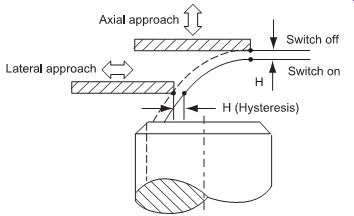
FIG. 1.46: Switching hysteresis.

To measure the maximum switching frequency, two tests (performed in accordance with EN 60947-5-2) enable the maximum switching frequency

f = l/(t1 + t2)

to be determined exactly from the duration of the "switch ON" period (t1) and the "switch OFF" period (t2). (See FIG. 1.47.)

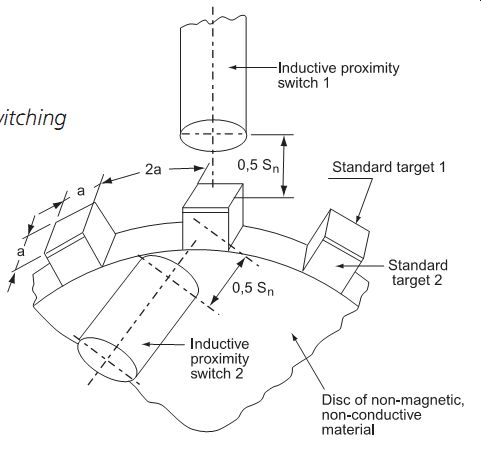
FIG. 1.47: Measuring maximum switching frequency.

Most DC versions employ normally open, normally closed or changeover circuitry and are available with either NPN or PNP open collector outputs.

¦ Operating voltage (VB)

A 5% residual ripple must not cause the operating voltage to fall below the minimum stated value. Correspondingly, a 10% ripple must not cause the operating voltage to exceed the maximum value quoted.

¦ Voltage drop (Vd)

Maximum voltage drop at the proximity switch if the output drops to zero.

¦ Residual voltage (Vr)

Voltage drop at the load if the sensing output is not conducting.

¦ Maximum load current (la)

Under nominal conditions, the output of the proximity switch cannot be driven by a current greater than this value.

¦ Residual current (lr)

If the output is not conducting, Ir is the maximum current flowing through the load.

¦ Current consumption without load (lo)

Current consumption of the switch under nominal conditions without load.

¦ Standby delay (tv)

Period between the application of the operating voltage and the sensor reaching the "ready" state. It is determined by the transient behavior of the oscillator.

¦ Series and parallel circuitry

If required, inductive proximity switches can be connected in series or in parallel. For series connection, the voltage drops Vd of two or more 3-wire switches (DC) or 2-wire switches (AC or DC) can be significant. Care should be taken that the output voltage is large enough to drive the load. With the NPN-version, the 3-wire switches must be connected to a common positive terminal. With the PNP-version, connect the switches to a common negative terminal. Series connection results in an AND function.

Parallel connection of 2-wire switches (AC) and 3-wire switches (DC) with open collector outputs is possible. The sum of the residual currents must be negligible enough to prevent the load (the holding current of a relay or magnetic switch) from being activated. For 3-wire switches with a collector resistor, it is recommended to decouple the sensing outputs with diodes. An OR function is obtained by connecting the switches in parallel.

Logic cards can be added to inductive proximity sensors. They receive the proximity sensor signal, amplify it and modify the output to respond in a particular way (as determined by time delay, pulse, or other logic). Besides operating output devices, the logic card output signal can be used as input to another card for customer logic. This is done most often with a modular control base.

One-shot (pulsed) logic gives a single fixed pulse in response to a change at the sensor. This is often used as a leading edge detector for moving parts, where the first indication of presence requires a single operation to take place, but where the continued presence will not cause recycling to occur.

Maintained (latching) logic might be used to detect parts for manual reject. The out put is continuous until the operator resets. After resets, the output will not trigger if the original target is still in front of the sensor.

ON delay does not trigger immediately with a change at the sensor, but will trigger only if the input signal exceeds a preset time delay. For example, it can provide jam-up detection on a conveyor for parts feeding at specific intervals. A slow down or stoppage downstream will cause a slower rate of passage, recognized as overloading or jam-up, and will cause an output to give warning or shut down the equipment until the cause is eliminated. A similar type provides an output which stays ON even when the cause is corrected, until manually reset by the operator.

ON/OFF delay is used especially for jam-up detection on vibration feeders and conveyors. The ON delay detects a jam-up, and the OFF delay allows the needed time for the jam to clear the sensing area.

Zero-speed detection provides shutdown for universal jam-up detection where the product may end up in front of the sensor for too long an interval, depending on whether the jam is upstream or downstream. If the interval exceeds a preset time, the output turns OFF or shuts down the equipment.

Photoelectric Sensors

Photoelectric sensors respond to the presence of all types of objects, be it large or small, transparent or opaque, shiny or dull, static or in motion. They can sense targets from distances of a few millimeters up to 100 meters. Photoelectric sensors use an emitter unit to produce a beam of light that is detected by a receiver. When the beam is broken, a "presence is detected.

The emitter light source is a modulated, vibration-resistant LED. This beam, which may be infrared, visible red or green, is switched at high currents for short time intervals so as to generate a high-energy pulse to provide long scanning distances or penetration in severe environments. Pulsing also means low power consumption.

The receiver contains a phototransistor that produces a signal when light falls upon it. A phototransistor is used because it has the best spectral match to the LED, a fast response, and is temperature stable. By tuning the receiver circuitry to respond to a narrow band around the LED pulsing frequency, very high ambient light and noise rejection can be achieved. Tuning the receiver to respond only to a specific phase of the pulsed beam can further enhance this effect.

The availability of various fiber optic cables with sensing elements permits photoelectric sensors to be used in many applications where space is limited or where there is a hazardous environment. These sensors also are capable of sensing objects traveling at high speeds with the option of detection at up to 8 kHz if necessary.

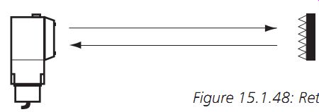
FIG. 1.48: Retroreflective scanning.

Selecting and Specifying Photoelectric Sensors

There are different scanning techniques available for photoelectric controls. Retroreflective scanning uses an emitter and receiver housed in the same unit with the beam reaching the receiver via a reflector (FIG. 1.48). Advantages are single side mounting, easy alignment and the ability to mount a reflector in spaces too small for a receiver unit. Reflectors are either acrylic discs or panels, or reflective tape cut to a convenient size. The larger the reflector, the more light reaches the receiver, giving longer scanning distances.

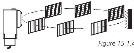
FIG. 1.49: Polarized scanning.

Polarized scanning involves all the features of retroreflective scanning with the addition of a polarized lens (FIG. 1.49). When the light wave hits the prismatic reflector, it is turned 90 degrees and, on return, allowed to pass through the receiving lens. This prevents false reflections when detecting shiny surfaces.

To reliably activate retroreflective and polarized scanning techniques, approximately 80 percent of the effective beam needs to be blocked. (See FIG. 1.50.) The diameter of the effective beam is the same as the reflector on one end and the lens of the photoelectric.

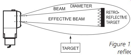
FIG. 1.50: Effective beam for retro reflective and polarized scanning.

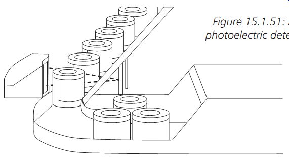
FIG. 1.51: A polarized retro reflective photoelectric detects highly reflective objects.

Using polarized retroreflective photoelectrics, highly reflective objects (FIG. 1.51) are detected for conveyor control. Polarized controls respond only to corner-cubed reflectors and ignore light reflected from the target, ensuring that the target always blocks the beam.

In automated assembly, the proper orientation of parts can be controlled by memorizing the reflectivity difference of the target sides. With the microprocessor-based photoelectric in FIG. 1.52, this is achieved by simply pushing an auto-tuning button.

With a through-scan technique (FIG. 1.53), the emitter and receiver are separate and positioned opposite one another, so that the light from the emitter shines directly on the receiver. This scanning mode gives maximum reliability (little chance of false reflections to the receiver), high penetration in contaminated environments, and long scanning distances. When installing adjacent through-scan systems, the emitter of one should be positioned next to the receiver of the next, to avoid one system detecting light from the other.

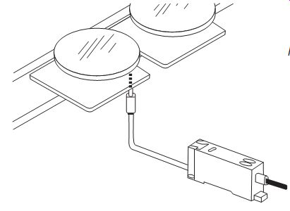
FIG. 1.52: A microprocessor based photoelectric memorizes reflectivity differences on target.

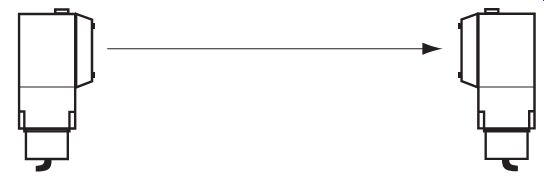
FIG. 1.53: Through scanning.

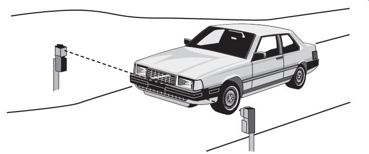
FIG. 1.54: Long distance, harsh duty photoelectrics withstand outdoor environments to solve such applications as traffic control at toll ways and automatic security gates.

To reliably activate through scanning, approximately 80 percent of the effective beam needs to be blocked. The diameter of the effective beam is the same size as the emitter and receiver lenses as shown in FIG. 1.55.

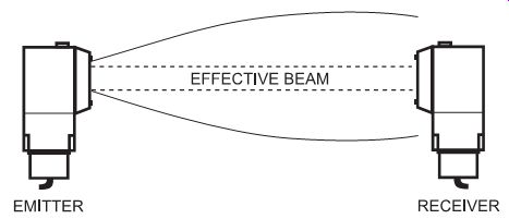
FIG. 1.55: Effective beam for through scanning.

In diffuse scanning, the emitter and receiver share the same housing, and the emitted beam is reflected to the receiver directly from the target (FIG. 1.56). This mode is used in cases where it is impractical to use a reflector, due to space considerations or when detection of a specific target is required. Because the reflected light is diffuse, a cleaner environment is necessary and scanning distances are shorter. The maximum scan distance of a diffuse-scan sensor is rated to a 10 × 10 cm white card. If the actual target is less reflective than a white card, the scan distance will be reduced. If the tar get is more reflective, the distance will be increased.

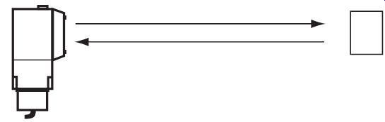
FIG. 1.56: Diffuse scanning.

Diffuse with background suppression is a special variety of diffuse scan. Using dual receivers and adjustable optics, targets can be reliably detected while backgrounds directly behind the targets are ignored (FIG. 1.58). They can be very useful when dark-colored objects are placed in front of highly reflective backgrounds (stainless steel, white conveyors, etc.).

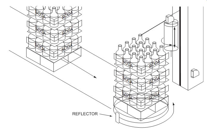
FIG. 1.57: Polarized and diffuse photoelectrics with time delays are used to detect both the presence and the height of the target to control wrapping on this palletizing and wrapping machine.

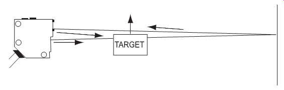
FIG. 1.58: Diffuse scanning with background suppression.

A convergent beam is another special variety of diffuse scan. Special lenses converge the beams to a fixed focal point in front of the control (FIG. 1.59). Convergent beams are useful for product positioning and ignoring background reflections. Convergent beams using visible red or green light produce a concentrated, small light spot on the target that can be used to detect color marks. Targets are detected within the "sensing window" of convergent beam controls. This window will increase with targets of higher reflectivity and decrease with targets of lower reflectivity.

Fiber optic photoelectric sensors use either through scan or diffuse scan fiber optic cables (FIG. 1.61). These cables allow sensing in very space-restricted areas and provide detection of very small targets. Cables are available with either plastic or glass fibers that the user can cut to length. Glass and stainless steel cables provide rugged protection and high-temperature capability. Many different cable end tips help solve many different applications.

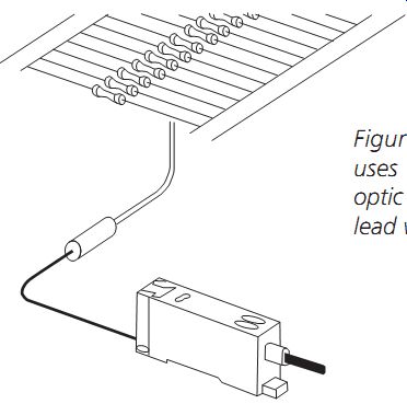
FIG. 1.62: A photoelectric sensor uses a small diameter diffuse scan fiber optic cable to detect electronic component lead wires.

The specified scanning distance for a photoelectric sensor is the guaranteed minimum operating distance in a clean environment. For retroreflective units, this distance is that obtained using a reflector of 100 percent efficiency. For diffuse units, this distance is that obtained using white Kodak paper with specified dimensions, usually 10 × 10 cm. Use of other materials affects the diffuse scanning distance as follows:

¦ Kodak white paper, 100%

¦ Aluminum, 120-150%

¦ Brown Kraft paper, 60-70%

Response time is the time between optical change of the system and the output changing to ON or OFF.

Frequency of operation is measured in cycles per second (Hz) and is calculated by:

Frequency of Operation = 1

(Response time ON + Response time OFF)

Interfacing and Design Information for Photoelectric Sensors

Photoelectric sensors have light and dark operation (LO/DO) modes. In LO, the out put is ON when light is incident on the receiver and OFF when there is no light at the receiver; in DO, the output is ON when there is no light incident on the receiver and OFF when there is light at the receiver.

Today, many photoelectric sensors have self-diagnostic LED indicators and outputs.

Most are equipped with LED indicators that provide early warning of malfunctions due to misalignment or contaminants on the lens surface. Generally, the LEDs indicate a stable light or unstable light condition (see FIG. 1.63).

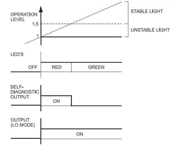
FIG. 1.63: LEDs indicate stable and unstable light conditions.

Stable light: The Green LED illuminates to show that the photoelectric is receiving at least 1.5 times the minimum operating light level of the sensor (normal operation).

Unstable light: The Green LED changes to Red (or turns OFF) to show that the photoelectric is receiving an amount of light less than 50% extra but still greater than the minimum operating point. The sensor is still operating but marginally.

Certain photoelectric sensors also are equipped with an additional wire that provides a remote self-diagnostic output. This output activates when the sensor is operating in the unstable light condition. This signal can be connected to a PLC or directly to an alarm circuit to inform an user at a remote location about an unstable sensor. Adjustment to the sensor (cleaning the lens, realignment, etc.) can then be made to prevent downtime.

Some newer photoelectrics have LED indicators that provide information on the both the "dark" conditions as well as the "light" conditions. On these sensors, the Green LED indicates whether the sensor is operating in a stable dark or unstable dark condition in addition to stable and unstable light (FIG. 1.64).

Stable dark: The Green LED illuminates to show that the emitted light beam is fully blocked from the receiving element of the photoelectric (normal operation).

Unstable dark: The Green LED turns OFF to show that some light is still reaching the photoelectric receiver. It is not a level high enough to operate the sensor, but it is a marginal condition. If the marginal condition continues for one full cycle of operation, the Green LED will flicker and activate a remote self diagnostic output.

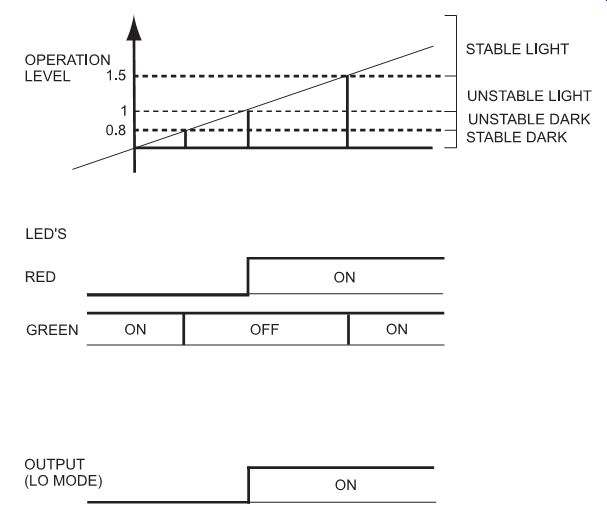
FIG. 1.64: LEDs also can indicate stable or unstable darkness.

Latest and Future Developments

Position sensors indicate the precise location of an object, a defined target or even a human being to control a surrounding process or improve its effectiveness. New electronic parts have improved the overall characteristics of sensors, and more functionality is being added at the sensor level. Diagnostic functions and easy-to-use calibration features are improving control systems and reducing installation time.

Communication modes are increasingly important in determining the right sensing technology for an application, and the ability of manufacturers to offer a combination of technologies is a major advantage. The focus is and will be on the application and how to best solve it. Sensing technology is the enabler and, therefore, the emphasis should not be on the technology itself but on the most effective way to meet the needs of the application.

The demand for communications, especially the ability to receive real-time data from remote locations to improve process control, continues to grow. Wireless technology is a "hot" topic as it significantly improves the flow of real-time data. It is quite possible that in the near future, sensors will not only be able to communicate to remote control areas, but also start communicating amongst themselves. Some local control loops will also be available to optimize processes and ensure that quality and safety standards are being met at all times.

References and Resources (PDFs)

"Hall Effect Sensing and Application," Honeywell, Inc.

"Applying Linear Output Hall Effect Transducers," Honeywell, Inc.

"Current Sink and Current Source Interfacing for Solid State Sensors," Honeywell, Inc.

"Interfacing Digital Hall Effect Sensors," Honeywell, Inc.

"Interpreting Operating Characteristics for Solid State Sensors," Honeywell, Inc.

"Gear Tooth Sensor Target Guidelines," Honeywell, Inc.

"Magnet Conversion Chart," Honeywell, Inc.

"Magnets," Honeywell, Inc.

"Method of Magnet Actuation," Honeywell, Inc.

" Solid State Sensors Glossary of Terms," Honeywell, Inc.

2. String Potentiometer and String Encoder Engineering Guide

This section reviews the advantages and disadvantages of string potentiometers and string encoders, hereafter referred to as CPTs (cable position transducers). Other names often used to refer to these transducers are:

¦ cable actuated position sensor

¦ cable extension transducer

¦ cable position transducer

¦ cable sensor

¦ cable-actuated sensor

¦ CET

¦ CPT

¦ stringpot

¦ string potentiometer

¦ draw wire encoder

¦ draw wire transducer

¦ wire rope transducer

¦ wire sensor

¦ wire-actuated transducer

¦ yo yo pot

¦ yo yo potentiometer

These names all refer to devices that measure displacement via a flexible displacement cable that extracts from and retracts to a spring-loaded drum. This drum is attached to a rotary sensor (see FIG. 2.1). By understanding the strengths and weaknesses of CPT technology, designers, engineers, and technicians can specify and design the best displacement measurement solution for their application.

Technology Review

CPTs were first developed in the mid 1960s in concert with the growth of the aerospace and aircraft industries. The first applications involved the monitoring of aircraft flight control mechanisms during flight testing.

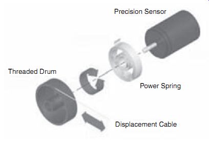
FIG. 2.1: How CPTs work.

While the technology is proven and mature, it is certainly not dated. A broad range of high-performance and cost-conscious applications use CPTs as the basis for key control and monitoring operations. Recent examples include:

¦ Delta IV missile thrust vectoring system

¦ Military fighter level sensor

¦ Diesel engine fuel index measurement

¦ International Space Station environmental control systems

¦ commercial and military aircraft flight data recorder input sensors

¦ excavator hydraulic cylinder control

¦ medical table actuation feedback system

¦ V-22 flight control surface monitoring

¦ Global Hawk UAV landing gear stroke measurement

¦ logistics sorting and positioning equipment

¦ earth borer positioner

Advantages of CPTs

CPTs have numerous advantages over other types of position sensors:

Multi-axis Capability. As FIG. 2.2 below shows, CPTs can be used to track linear, rotary, 2-dimensional, and 3-dimensional displacements. This capability makes CPTs ideal in test engineering as well as in OEM applications where size and mounting restrictions eliminate other choices.

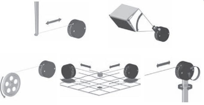
FIG. 2.2: Linear, angular, rotary, 2D, and 3D displacements can be monitored with CPTs.

Flexible Mounting. The flexible displacement cable inherent in CPT technology al lows for flexible mounting. The cable can be attached to the application in a number of ways as shown in FIG. 2.3. Other methods include magnets and eyebolts or other threaded fasteners.

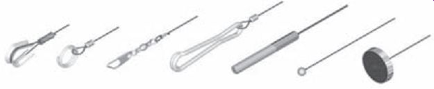
FIG. 2.3: A few displacement cable terminations.

The cable can also be routed around barriers using pulleys (see FIG. 2.4) and

flexible conduits.

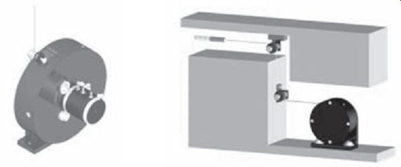
FIG. 2.4: Pulleys and idlers allow displacement cable to be routed to the application.

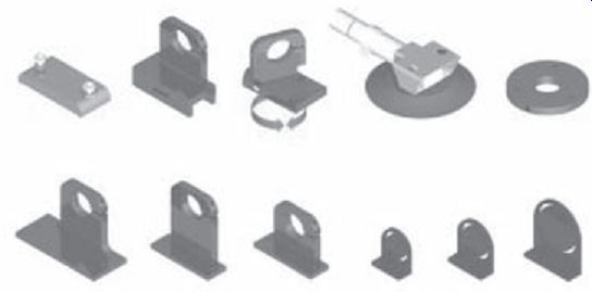
FIG. 2.5: A few mounting base options.

Finally, innovative transducer mounting bases and cable exit options (see Figures 2.5 and 2.6) give additional mounting flexibility, eliminating the expense associated with special fixturing and adapters.

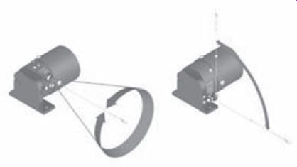
FIG. 2.6: Cable exit choices provide ease of installation and application flexibility.

Fast Installation. The flexible mounting features combined with the broad tolerance for displacement cable misalignment provide for fast installation, often in less than 2 minutes (see FIG. 2.7). This reduces installation costs and can be particularly valuable in test and research and development applications.

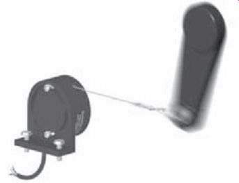
FIG. 2.7: Installation is fast.

Small Size. CPT technology gives the user a small size relative to measurement range. The world's smallest CPT measures a 1.5 inches (38.1 mm) displacement with a size of only 0.75 inch square by 0.38 inch (19 mm × 19 mm × 10 mm) as shown in FIG. 2.8. As the measurement range increases, the CPT's relative small size advantage becomes more obvious as shown in FIG. 2.9.

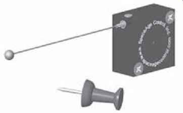
FIG. 2.8: World's smallest CPT: The Series 150.

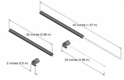
FIG. 2.9: Size comparison of CPTs to rod-and-cylinder devices such as LVDTs and linear potentiometers.

Lightweight. CPTs measure displacement with a reliable, low mass stainless steel or high-strength fabric-based cable. This feature along with generally anodized aluminum components results in a product that has a low-weight-to-range ratio. This benefit can be important in space, missile, aircraft, racing, robotic, and biomedical applications. Low mass can also increase survivability in high shock and vibration environments encountered in industrial machinery and equipment applications. Table 2.1 shows a comparison of weight to range for various displacement measurement sensors.

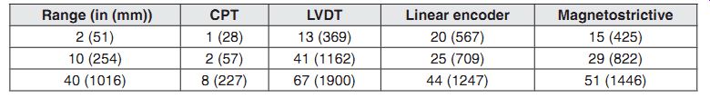
Table 2.1: CPTs have a weight-to-range advantage over other sensor types (mass shown in oz (g)).

Rugged. Properly designed and manufactured CPTs have performed reliably for over 35 years in harsh industrial, aerospace, testing, and outdoor environments. The design of CPTs can be mechanically and electrically simple, resulting in high reliability, low maintenance, and years of service. CPT environmental testing has demonstrated the effective operation of CPTs in environments containing high shock, vibration, humidity, corrosion, moisture, and other parameters.

Variety of Electrical Outputs. What does your controller or data acquisition device require?

4-20 mA? 0 to 5 VDC? 0 to 10 VDC? ±5 VDC? ±10 VDC?

Strain gage compatible? Quadrature? RS-232? LVDT or RVDT type signals? Synchro or resolver type signals? Because CPTs can incorporate a broad range of rotary sensors and related signal conditioning, the electrical output of your choice is typically available.

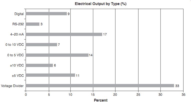
FIG. 2.10: Typical electrical output by frequency of use.

Low Power, Simple Signal Conditioning. CPTs, particularly analog potentiometer types, generally have low power and simple signal conditioning requirements. 5 VDC power or less is suitable and no special signal conditioning is required for the majority of applications. The CPT signal input and output requirements can reduce total system cost, allow for fast setup, and allows for relatively inexperienced personnel to work with the devices.

Unobtrusive. The small size and low mass of CPTs give them a small profile. This provides for aesthetically pleasing designs. Additionally, this unobtrusiveness reduces the possibility for unwanted application interaction (accidental interference) with the transducer. Finally, the displacement cable can be designed to "break away" in applications where it is paramount that sensor failure does not interfere with the measured object. This can be quite important in flight control applications where flight safety can be affected if a failure of sensor's actuation mechanism makes it impossible for the aircraft to be properly controlled.

Broad Operating Temperature. Analog-output CPTs can operate in temperate ranges from -65°C to +125°C while digital-output CPTs can range from -40°C to +85°C or -20°C to +100°C. This broad operating range reduces operating and installation issues and makes the products well-suited for outdoor, aerospace, and industrial control applications. Broader operating ranges can be attained with the use of custom sensors.

Accuracy. Using non-backlash connections and threaded drums, analog-output CPTs can offer linearity-compensated accuracy exceeding ±0.025% of full scale. As an example, a 10-inch (254-mm) range analog-output CPT can give an accuracy of ±0.0025 inch (±0.0635 mm).

Broad Measurement Range. CPTs measurement ranges are broad: 1.5 inches to over 2000 inches (38 mm to over 50 m). For some long-range measurement challenges, the CPT is the only feasible solution.

Cost Effective. CPTs are generally cost-effective devices, especially when considering lifetime costs. Flexible mounting, fast installation, high reliability, and minimal signal conditioning requirements reduce costs relative to many alternatives. The CPT's cost effectiveness increases at longer ranges because the displacement cable is the primary cost adder to the design in going from shorter ranges to longer ranges.

Other Design Factors

There is no perfect sensing technology. CPTs are no exception. Even Superman has his Kryptonite. When considering a CPT for an application, keep the following items in mind:

Frequency Response. CPTs are used extensively in vehicle impact testing where accelerations exceed 50 g's. CPTs have been used in other applications where accelerations approach 100 g's. However, applications involving extreme acceleration can exceed the frequency response capabilities of CPTs. Examples where CPT frequency response can be an issue include applications that require cable accelerations in ex cess of 100 g's and environments using analog-output CPTs with very high frequency, low displacement motion that tends to cause dithering wear of the potentiometric element. During extreme high accelerations, it is possible the cable reel's inertia and the power spring's insufficient torque will cause the reel to rotate to a point where the displacement cable goes slack.

Lifetime. CPTs with optical encoder or conductive plastic sensing technologies can operate in excess of 100 million shaft revolutions. However, longer range analog output CPTs require multi-turn potentiometers with lifetimes of less than 10 million shaft revolutions. While long-displacement, high-cycle applications are not common, you should do a thorough cost and reliability analysis before specifying a CPT for this type of use.

Cable Tension on Application. Non-contact sensing devices such as ultrasonic, Hall effect, or laser do not mechanically affect the application. The CPT's cable tension imparts a load on the application. While this load can be minimized to as little as 1 oz. (0.278 N), it cannot be eliminated. Hence, for applications sensitive to external loads, other technologies should be considered.

Cable Interference. The CPT's small, lightweight displacement cable is one of its key advantages. In some applications, it can be a disadvantage. For example, inadvertent damage can occur if technicians and operators do not know of the cable's presence. While signage and protective tubing or other devices can be installed, dam age can still occur from unplanned events.

Accuracy. CPTs that use no-backlash mechanical connections and threaded drums deliver excellent accuracy. Nevertheless, this is sometimes insufficient for some applications. For those situations, you should consider using LVDTs, laser-based devices, or other higher-accuracy technologies.

Accuracy is a broadly-used yet not always fully defined word. When you are determining what "accuracy" you require for your application, ensure you really need the accuracy you are specifying. See if your application does not require raw accuracy but rather good linearity, resolution, repeatability, or hysteresis.

Catenary Curve Error Effects. A catenary curve describes the shape the displacement cable takes when subjected to a uniform force such as gravity. Because the mass of the cable per unit length is so small and the cable tension is relatively high, cable sag does not produce any significant error unless the cable length is exceptionally long (over 60 feet (18 meters)). The cable sag error is minor compared to other error sources (generally less than ± 0.0025%). Nevertheless, some applications, (typically involving high angular rotation or long measurements), produce sufficient forces to cause significant cable sag error. To calculate the catenary curve error effect for your application, visit http://spaceagecontrol.com/calccabl.htm.

Conclusion

Cable position transducers can be flexible, robust, cost-effective displacement measurement devices for a broad range of applications. At the same time, these products have limitations that may result in other technologies being more appropriate for specific applications.

Reference Materials

These documents provide additional information on the selection and use of CPTs:

¦ Application Note for Aircraft/Aerospace (S004A) http://spaceagecontrol.com/s004a.pdf

¦ Application Note for Ground Vehicles/Transportation (S005A) http://spaceagecontrol.com/s005a.pdf

¦ Selecting Position Transducers http://spaceagecontrol.com/selpt.htm

¦ Sensor and Transducer Total Cost of Ownership (S054A) http://spaceagecontrol.com/s054a.htm

The LVDT (see FIG. 3.2) is a position-to-electrical sensor whose output is proportional to the position of a movable magnetic core. The core moves linearly inside a transformer consisting of a center primary coil and two outer secondary coils wound on a cylindrical form. The primary winding is excited with an AC voltage source (typically several kHz), inducing secondary voltages which vary with the position of the magnetic core within the assembly. The core is usually threaded in order to facilitate attachment to a nonferromagnetic rod which in turn in attached to the object whose movement or displacement is being measured.

The secondary windings are wound out of phase with each other, and when the core is centered the voltages in the two secondary windings oppose each other, and the net output voltage is zero. When the core is moved off center, the voltage in the secondary toward which the core is moved increases, while the opposite voltage decreases. The result is a differential voltage output which varies linearly with the core's position.

Linearity is excellent over the design range of movement, typically 0.5% or better.

The LVDT offers good accuracy, linearity, sensitivity, infinite resolution, as well as frictionless operation and ruggedness.

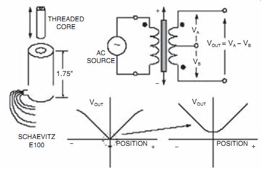
FIG. 3.2: Linear variable differential transformer (LVDT).

A wide variety of measurement ranges are available in different LVDTs, typically from ±100 µm to ±25 cm. Typical excitation voltages range from 1 V to 24 V rms, with frequencies from 50 Hz to 20 kHz. Key specifications for the Schaevitz E100 LVDT are given in FIG. 3.3.

-------------

¦ Nominal Linear Range: ±0.1 inches (± 2.54 mm)

¦ Input Voltage: 3V rms

¦ Operating Frequency: 50 Hz to 10 kHz (2.5 kHz nominal)

¦ Linearity: 0.5% Fullscale

¦ Sensitivity: 2.4 mV Output / 0.001 inches / Volt Excitation

¦ Primary Impedance: 660?

¦ Secondary Impedance: 960?

FIG. 3.3: Schaevitz E100 LVDT specifications.

--------------

Note that a true null does not occur when the core is in center position because of mismatches between the two secondary windings and leakage inductance. Also, simply measuring the output voltage VOUT will not tell on which side of the null position the core resides.

A signal conditioning circuit which removes these difficulties is shown in FIG. 3.4 where the absolute values of the two output voltages are subtracted. Using this technique, both positive and negative variations about the center position can be measured. While a diode/capacitor-type rectifier could be used as the absolute value circuit, the precision rectifier shown in FIG. 3.5 is more accurate and linear. The input is applied to a V/I converter which in turn drives an analog multiplier. The sign of the differential input is detected by the comparator whose output switches the sign of the V/I output via the analog multiplier. The final output is a precision replica of the absolute value of the input. These circuits are well understood by IC designers and are easy to implement on modern bipolar processes.

The industry-standard AD598 LVDT signal conditioner shown in FIG. 3.6 (simplified form) performs all required LVDT signal processing. The on-chip excitation frequency oscillator can be set from 20 Hz to 20 kHz with a single external capacitor.

Two absolute value circuits followed by two filters are used to detect the amplitude of the A and B channel inputs. Analog circuits are then used to generate the ratiometric function [A-B]/[A+B]. Note that this function is independent of the amplitude of the primary winding excitation voltage, assuming the sum of the LVDT output volt age amplitudes remains constant over the operating range. This is usually the case for most LVDTs, but the user should always check with the manufacturer if it is not specified on the LVDT data sheet. Note also that this approach requires the use of a 5-wire LVDT.

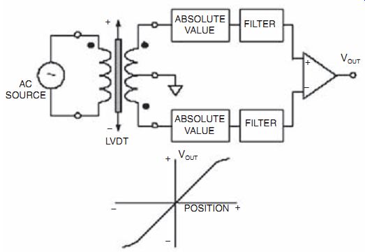
FIG. 3.4: Improved LVDT output signal processing.

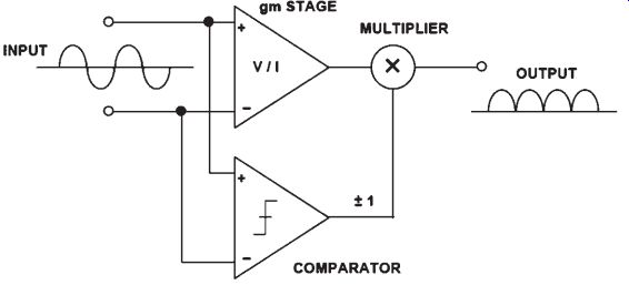
FIG. 3.5: Precision absolute value circuit (full-wave rectifier).

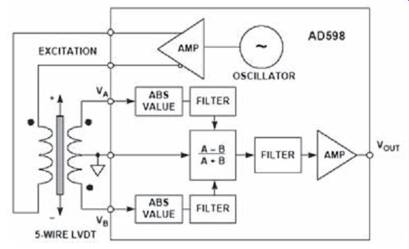
FIG. 3.6: AD598 LVDT signal conditioner (simplified).

A single external resistor sets the AD598 excitation voltage from approximately 1 V rms to 24 V rms. Drive capability is 30 mA rms. The AD598 can drive an LVDT at the end of 300 feet of cable, since the circuit is not affected by phase shifts or absolute signal magnitudes. The position output range of VOUT is ±11 V for a 6 mA load and it can drive up to 1000 feet of cable. The VA and VB inputs can be as low as 100 mV rms.

The AD698 LVDT signal conditioner (see FIG. 3.7) has similar specifications as the AD598 but processes the signals slightly differently. Note that the AD698 operates from a 4-wire LVDT and uses synchronous demodulation. The A and B signal processors each consist of an absolute value function and a filter. The A output is then divided by the B output to produce a final output which is ratiometric and independent of the excitation voltage amplitude. Note that the sum of the LVDT secondary voltages does not have to remain constant in the AD698.

The AD698 can also be used with a half-bridge (similar to an auto-transformer)

LVDT as shown in FIG. 3.8. In this arrangement, the entire secondary voltage is applied to the B processor, while the center-tap voltage is applied to the A processor.

The half-bridge LVDT does not produce a null voltage, and the A/B ratio represents the range-of-travel of the core.

It should be noted that the LVDT concept can be implemented in rotary form, in which case the device is called a rotary variable differential transformer (RVDT). The shaft is equivalent to the core in an LVDT, and the transformer windings are wound on the stationary part of the assembly. However, the RVDT is linear over a relatively narrow range of rotation and is not capable of measuring a full 360° rotation. Al-though capable of continuous rotation, typical RVDTs are linear over a range of about ±40° about the null position (0°). Typical sensitivity is 2-3 mV per volt per degree of rotation, with input voltages in the range of 3 V rms at frequencies between 400 Hz and 20 kHz. The 0° position is marked on the shaft and the body.

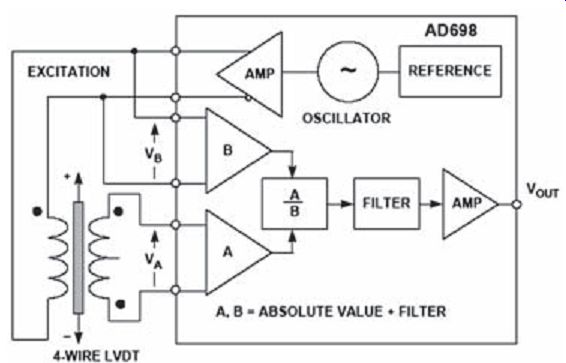
FIG. 3.7: AD698 LVDT signal conditioner (simplified).

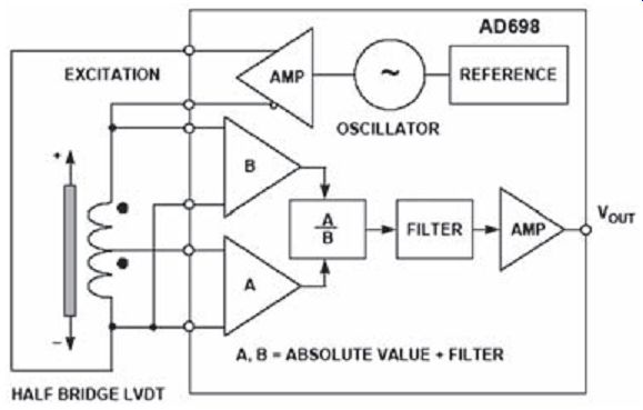
FIG. 3.8: Half-bridge LVDT configuration.

FIG. 3.9: Hall effect sensors.

Hall Effect Magnetic Sensors

If a current flows in a conductor (or semiconductor) and there is a magnetic field present which is perpendicular to the current flow, then the combination of current and magnetic field will generate a voltage perpendicular to both (see FIG. 3.9). This phenomenon, called the Hall Effect, was discovered by E. H. Hall in 1879. The voltage, VH, is known as the Hall Voltage.

VH is a function of the current density, the magnetic field, and the charge density and carrier mobility of the conductor.

As discussed earlier in this SECTION and elsewhere in this handbook, he Hall effect may be used to measure magnetic fields (and hence in contact-free current measurement), but its commonest application is in motion sensors where a fixed Hall sensor and a small magnet attached to a moving part can replace a cam and contacts with a great improvement in reliability. (Cams wear and contacts arc or become fouled, but magnets and Hall sensors are contact free and do neither.)

Since VH is proportional to magnetic field and not to rate of change of magnetic field like an inductive sensor, the Hall effect provides a more reliable low-speed sensor than an inductive pickup.

Although several materials can be used for Hall effect sensors, silicon has the advantage that signal conditioning circuits can be integrated on the same chip as the sensor.

CMOS processes are common for this application. A simple rotational speed detector can be made with a Hall sensor, a gain stage, and a comparator as shown in FIG. 3.10. The circuit is designed to detect rotation speed as in automotive applications.

It responds to small changes in field, and the comparator has built-in hysteresis to pre vent oscillation. Several companies manufacture such Hall switches, and their usage is widespread.

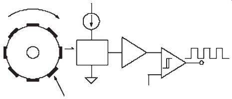
FIG. 3.10: Hall effect sensor used as a rotation sensor.

There are many other applications, particularly in automotive throttle, pedal, suspension, and valve position sensing, where a linear representation of the magnetic field is desired. The AD22151 is a linear magnetic field sensor whose output voltage is proportional to a magnetic field applied perpendicularly to the package top surface (see FIG. 3.11). The AD22151 combines integrated bulk Hall cell technology and conditioning circuitry to minimize temperature related drifts associated with silicon Hall cell characteristics.

The architecture maximizes the advantages of a monolithic implementation while al lowing sufficient versatility to meet varied application requirements with a minimum number of external components. Principal features include dynamic offset drift cancellation using a chopper-type op amp and a built-in temperature sensor. Designed for single +5 V supply operation, low offset and gain drift allows operation over a -40°C to +150°C range. Temperature compensation (set externally with a resistor R1) can accommodate a number of magnetic materials commonly utilized in position sensors.

Output voltage range and gain can be easily set with external resistors. Typical gain range is usually set from 2 mV/Gauss to 6 mV/Gauss. Output voltage can be adjusted from fully bipolar (reversible) field operation to fully unipolar field sensing. The voltage output achieves near rail-to-rail dynamic range (+0.5 V to +4.5 V), capable of supplying 1 mA into large capacitive loads. The output signal is ratiometric to the positive supply rail in all configurations.

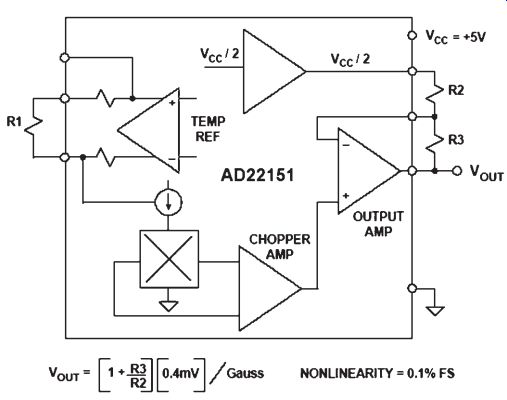
FIG. 3.11: AD22151 Linear output magnetic field sensor.

Optical Encoders

Among the most popular position measuring sensors, optical encoders find use in relatively low reliability and low resolution applications. An incremental optical encoder (left-hand diagram in FIG. 3.12) is a disc divided into sectors that are alternately transparent and opaque. A light source is positioned on one side of the disc, and a light sensor on the other side. As the disc rotates, the output from the detector switches alternately on and off, depending on whether the sector appearing between the light source and the detector is transparent or opaque. Thus, the encoder produces a stream of square wave pulses which, when counted, indicates the angular position of the shaft. Available encoder resolutions (the number of opaque and transparent sectors per disc) range from 100 to 65,000, with absolute accuracies approaching 30 arc-seconds (1/43,200 per rotation). Most incremental encoders feature a second light source and sensor at an angle to the main source and sensor, to indicate the direction of rotation. Many encoders also have a third light source and detector to sense a once per-revolution marker. Without some form of revolution marker, absolute angles are difficult to determine. A potentially serious disadvantage is that incremental encoders require external counters to determine absolute angles within a given rotation. If the power is momentarily shut off, or if the encoder misses a pulse due to noise or a dirty disc, the resulting angular information will be in error.

The absolute optical encoder (right-hand diagram in FIG. 3.12) overcomes these disadvantages but is more expensive. An absolute optical encoder's disc is divided up into N sectors (N = 5 for example shown), and each sector is further divided radially along its length into opaque and transparent sections, forming a unique N-bit digital word with a maximum count of 2N - 1. The digital word formed radially by each sector increments in value from one sector to the next, usually employing Gray code.

Binary coding could be used, but can produce large errors if a single bit is incorrectly interpreted by the sensors. Gray code overcomes this defect: the maximum error produced by an error in any single bit of the Gray code is only 1 LSB after the Gray code is converted into binary code. A set of N light sensors responds to the N-bit digital word which corresponds to the disc's absolute angular position. Industrial optical encoders achieve up to 16-bit resolution, with absolute accuracies that approach the resolution (20 arc seconds). Both absolute and incremental optical encoders, however, may suffer damage in harsh industrial environments.

Resolvers and Synchros

Machine-tool and robotics manufacturers have increasingly turned to resolvers and synchros to provide accurate angular and rotational information. These devices excel in demanding factory applications requiring small size, long-term reliability, absolute position measurement, high accuracy, and low-noise operation.

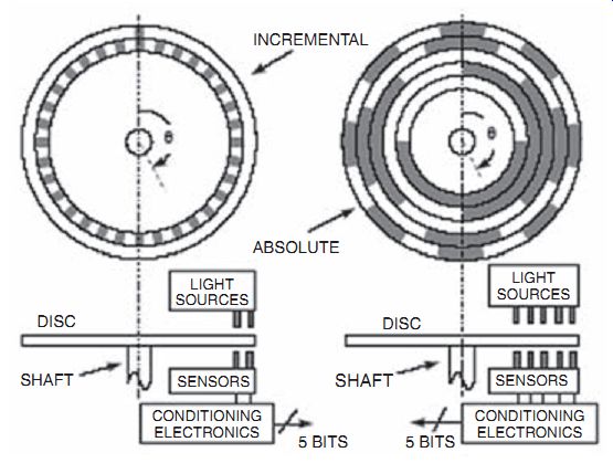
FIG. 3.12: Incremental and absolute optical encoders.

A diagram of a typical synchro and resolver is shown in FIG. 3.13. Both synchros and resolvers employ single-winding rotors that revolve inside fixed stators. In the case of a simple synchro, the stator has three windings oriented 120° apart and electrically connected in a Y-connection. Resolvers differ from synchros in that their stators have only two windings oriented at 90°.

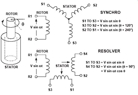
FIG. 3.13: Synchros and resolvers.

Because synchros have three stator coils in a 120° orientation, they are more difficult than resolvers to manufacture and are therefore more costly. Today, synchros find decreasing use, except in certain military and avionic retrofit applications.

Modern resolvers, in contrast, are available in a brushless form that employ a trans former to couple the rotor signals from the stator to the rotor. The primary winding of this transformer resides on the stator, and the secondary on the rotor. Other resolvers use more traditional brushes or slip rings to couple the signal into the rotor winding.

Brushless resolvers are more rugged than synchros because there are no brushes to break or dislodge, and the life of a brushless resolver is limited only by its bearings.

Most resolvers are specified to work over 2 V to 40 V rms and at frequencies from 400 Hz to 10 kHz. Angular accuracies range from 5 arc-minutes to 0.5 arc-minutes.

(There are 60 arc-minutes in one degree, and 60 arc-seconds in one arc-minute. Hence, one arc-minute is equal to 0.0167 degrees.)

In operation, synchros and resolvers resemble rotating transformers. The rotor winding is excited by an AC reference voltage, at frequencies up to a few kHz. The magnitude of the voltage induced in any stator winding is proportional to the sine of the angle, ?, between the rotor coil axis and the stator coil axis. In the case of a synchro, the voltage induced across any pair of stator terminals will be the vector sum of the voltages across the two connected coils.

For example, if the rotor of a synchro is excited with a reference voltage, Vsinfit, across its terminals R1 and R2, then the stator's terminal will see voltages in the form:

S1 to S3 = V sinfit sin?

S3 to S2 = V sinfit sin (? + 120°) S2 to S1 = V sinfit sin (? + 240°),

... where ohm is the shaft angle.

In the case of a resolver, with a rotor AC reference voltage of Vsinfit, the stator's terminal voltages will be:

S1 to S3 = V sinfit sin ?

S4 to S2 = V sinfit sin(? + 90°) = V sinfit cos?.

It should be noted that the 3-wire synchro output can be easily converted into the re solver-equivalent format using a Scott-T transformer. Therefore, the following signal processing example describes only the resolver configuration.

A typical resolver-to-digital converter (RDC) is shown functionally in FIG. 3.14.

The two outputs of the resolver are applied to cosine and sine multipliers. These multipliers incorporate sine and cosine lookup tables and function as multiplying digital-to-analog converters. Begin by assuming that the current state of the up/down counter is a digital number representing a trial angle, ?. The converter seeks to adjust the digital angle, ?, continuously to become equal to, and to track ?, the analog angle being measured. The resolver's stator output voltages are written as:

V1 = V sinfit sin?

V2 = V sinfit cos? where ohm is the angle of the resolver's rotor. The digital angle ohm is applied to the cosine multiplier, and its cosine is multiplied by V1 to produce the term:

V sinfit sin? cos?.

The digital angle ohm is also applied to the sine multiplier and multiplied by V2 to product the term:

V sinfit cos? sin?.

These two signals are subtracted from each other by the error amplifier to yield an AC error signal of the form:

V sinfit [sin? cos? - cos? sin?]. Using a simple trigonometric identity, this reduces to:

V sinfit [sin (? -?)].

The detector synchronously demodulates this AC error signal, using the resolver's rotor voltage as a reference. This results in a DC error signal proportional to sin(? - ?).

The DC error signal feeds an integrator, the output of which drives a voltage-con trolled-oscillator (VCO). The VCO, in turn, causes the up/down counter to count in the proper direction to cause:

sin (? - ?) ohm 0.

When this is achieved,

? - ohm ? 0, and therefore

? = ohm to within one count. Hence, the counter's digital output, ?, represents the angle ?. The latches enable this data to be transferred externally without interrupting the loop's tracking.

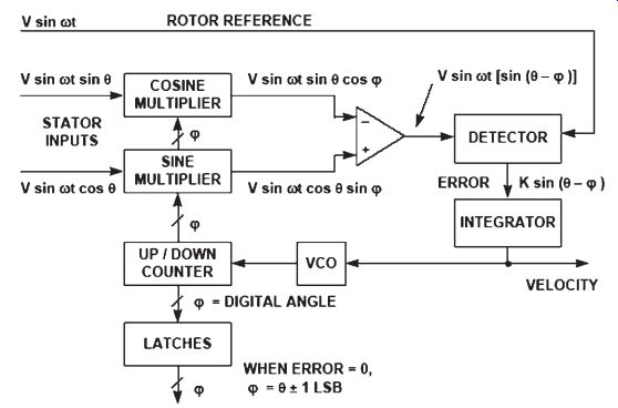
FIG. 3.14: Resolver-to-digital converter (RTD).

This circuit is equivalent to a so-called type-2 servo loop, because it has, in effect, two integrators. One is the counter, which accumulates pulses; the other is the integrator at the output of the detector. In a type-2 servo loop with a constant rotational velocity in put, the output digital word continuously follows, or tracks the input, without needing externally derived convert commands, and with no steady state phase lag between the digital output word and actual shaft angle. An error signal appears only during periods of acceleration or deceleration.

As an added bonus, the tracking RDC provides an analog DC output voltage directly proportional to the shaft's rotational velocity. This is a useful feature if velocity is to be measured or used as a stabilization term in a servo system, and it makes tachometers unnecessary.

Since the operation of an RDC depends only on the ratio between input signal amplitudes, attenuation in the lines connecting them to resolvers doesn't substantially affect performance. For similar reasons, these converters are not greatly susceptible to waveform distortion. In fact, they can operate with as much as 10% harmonic distortion on the input signals; some applications actually use square-wave references with little additional error.

Tracking ADCs are therefore ideally suited to RDCs. While other ADC architectures, such as successive approximation, could be used, the tracking converter is the most accurate and efficient for this application.

Because the tracking converter doubly integrates its error signal, the device offers a high degree of noise immunity (12 dB-per-octave rolloff). The net area under any given noise spike produces an error. However, typical inductively coupled noise spikes have equal positive and negative going waveforms. When integrated, this results in a zero net error signal. The resulting noise immunity, combined with the converter's insensitivity to voltage drops, lets the user locate the converter at a considerable distance from the resolver. Noise rejection is further enhanced by the detector's rejection of any signal not at the reference frequency, such as wideband noise.

The AD2S90 is one of a number of integrated RDCs offered by Analog Devices. Key specifications are shown in FIG. 3.15. The general architecture is similar to that of FIG. 3.14. The input signal level should be 2 V rms ± 10% in the frequency range from 3 kHz to 20 kHz.

FIG. 3.15: Performance characteristics for AD2S90 resolver-to-digital converter.

Inductosyns

Synchros and resolvers inherently measure rotary position, but they can make linear position measurements when used with lead screws. An alternative, the Inductosyn (registered trademark of Farrand Controls, Inc.) measures linear position directly. In addition, Inductosyns are accurate and rugged, well-suited to severe industrial environments, and do not require ohmic contact.

The linear Inductosyn consists of two magnetically coupled parts; it resembles a multipole resolver in its operation (see FIG. 3.16). One part, the scale, is fixed (e.g., with epoxy) to one axis, such as a machine tool bed. The other part, the slider, moves along the scale in conjunction with the device to be positioned (for example, the machine tool carrier).

The scale is constructed of a base material such as steel, stainless steel, aluminum, or a tape of spring steel, covered by an insulating layer. Bonded to this is a printed- circuit trace, in the form of a continuous rectangular waveform pattern. The pattern typically has a cyclic pitch of 0.1 inch, 0.2 inch, or 2 millimeters. The slider, about 4 inches long, has two separate but identical printed circuit traces bonded to the surface that faces the scale. These two traces have a waveform pattern with exactly the same cyclic pitch as the waveform on the scale, but one trace is shifted one-quarter of a cycle relative to the other. The slider and the scale remain separated by a small air gap of about 0.007 inch.

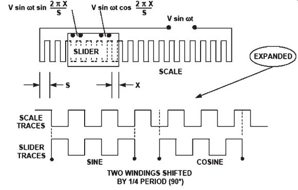
FIG. 3.16: Linear Inductosyn.

Inductosyn operation resembles that of a resolver. When the scale is energized with a sine wave, this voltage couples to the two slider windings, inducing voltages proportional to the sine and cosine of the slider's spacing within the cyclic pitch of the scale.

If S is the distance between pitches, and X is the slider displacement within a pitch, and the scale is energized with a voltage V sinfit, then the slider windings will see terminal voltages of:

V (sine output) = V sinfit sin[2pX/S]

V (cosine output) = V sinfit cos[2pX/S].

As the slider moves the distance of the scale pitch, the voltages produced by the two slider windings are similar to those produced by a resolver rotating through 360°. The absolute orientation of the Inductosyn is determined by counting successive pitches in either direction from an established starting point. Because the Inductosyn consists of a large number of cycles, some form of coarse control is necessary in order to avoid ambiguity. The usual method of providing this is to use a resolver or synchro operated through a rack and pinion or a lead screw.

In contrast to a resolver's highly efficient transformation of 1:1 or 2:1, typical Inductosyns operate with transformation ratios of 100:1. This results in a pair of sinusoidal output signals in the millivolt range which generally require amplification.

[...]

intervals, commutators wear and can be permanently damaged by inadequate brush maintenance, brush/commutator assemblies are a source of particulate contaminants, and the arcing of mechanical commutation can be a serious fire hazard is some environments.

The availability of power inverters capable of controlling high-horsepower motors allowed practical implementation of alternate motor architectures such as the DC permanent magnet synchronous motor (PMSM) in servo control applications. Although eliminating many of the mechanical problems associated with DC brush motors, these motors required more complex control schemes and suffered from several draw backs of their own. Aside from being costly, DC PMSMs in larger, high-horsepower configurations suffer from high rotor moment-of-inertia as well as limited use in high speed applications due to mechanical constraints of rotor construction and the need to implement field weakening to exceed baseplate speed.

In the 1960s, advances in control theory, in particular the development of indirect field-oriented control, provided the theoretical basis for dynamic control of AC induction motors. Because of the intensive mathematical computations required by indirect field-oriented control, now commonly referred to as vector control, practical implementation was not possible for many years. Available hardware could not perform the high-speed precision sensing of rotor position and near real-time computation of dynamic flux vectors. The current availability of precision optical encoders, isolated gate bipolar transistors (IGBTs), high-speed resolver-to-digital converters and high-speed digital signal processors (DSPs) has pushed vector control to the forefront of motor development due to the advantages inherent in the AC induction motor.

A simplified block diagram of an AC induction motor control system is shown in FIG. 3.17. In this example, a single-chip IC (ADMC300, ADMC330, or ADMC331) performs the control functions. The inputs to the controller chip are the motor cur rents (normally three-phase) and the motor rotor position and velocity. Hall-effect sensors are often used to monitor the currents, and a resolver and an RDC monitor the rotor position and velocity. The DSP is used to perform the real time vector-type calculations necessary to generate the control outputs to the inverter processors. The transformations required for vector control are also accomplished with the DSP.

The ADMC300 comprises a high performance, 5-channel 16-bit ADC system, a 12-bit 3-phase PWM generation unit, and a flexible encoder interface for position sensor feedback. The ADMC330 includes a 7-channel 12-bit ADC system and a 12-bit 3-phase PWM generator. The ADMC331 includes a 7-channel 12-bit ADC system, and a programmable 16-bit 3-phase PWM generator. It also has additional power factor correction control capabilities. All devices have on-chip DSPs (approximately 20 MHz) based on Analog Device's Modified Harvard Architecture 16-bit DSP core.

Third-party DSP software and reference designs are available to facilitate motor control system development using these chips.

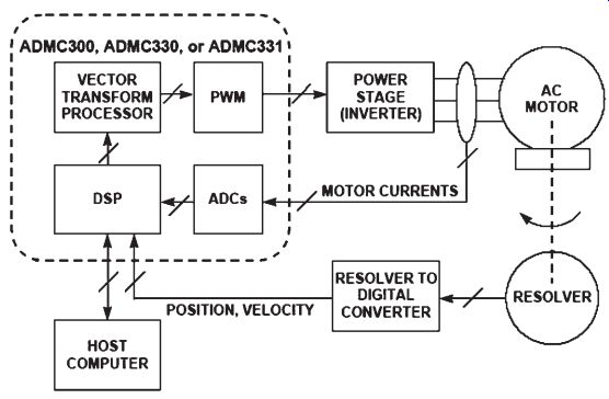
FIG. 3.17: AC induction motor control application.

Accelerometers

Accelerometers are widely used to measure tilt, inertial forces, shock, and vibration. They find wide usage in automotive, medical, industrial control, and other applications. Modern micromachining techniques allow these accelerometers to be manufactured on CMOS processes at low cost with high reliability. Analog Devices iMEMS® (Integrated Micro Electro Mechanical Systems) accelerometers represent a breakthrough in this technology. A significant advantage of this type of accelerometer over piezoelectric-type charge-output accelerometers is that DC acceleration can be measured (e.g., they can be used in tilt measurements where the acceleration is a constant 1g).

The basic unit cell sensor building block for these accelerometers is shown in FIG. 3.19. The surface micromachined sensor element is made by depositing poly silicon on a sacrificial oxide layer that is then etched away leaving the suspended sensor element. The actual sensor has tens of unit cells for sensing acceleration, but the diagram shows only one cell for clarity. The electrical basis of the sensor is the differential capacitor (CS1 and CS2) which is formed by a center plate which is part of the moving beam and two fixed outer plates. The two capacitors are equal at rest (no applied acceleration). When acceleration is applied, the mass of the beam causes it to move closer to one of the fixed plates while moving further from the other. This change in differential capacitance forms the electrical basis for the conditioning electronics shown in FIG. 3.20.

FIG. 3.18: Accelerometer applications.

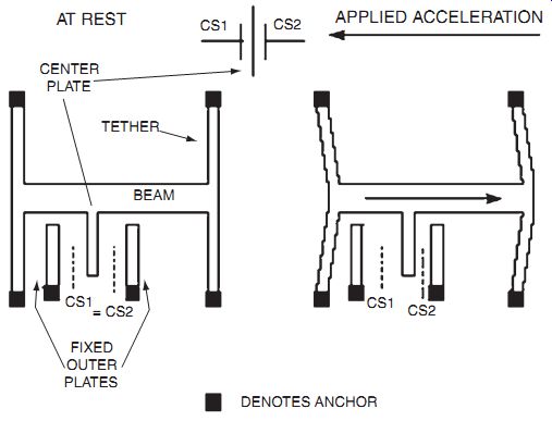
FIG. 3.19: ADXL-family micromachined accelerometers.

(Top view of IC.)

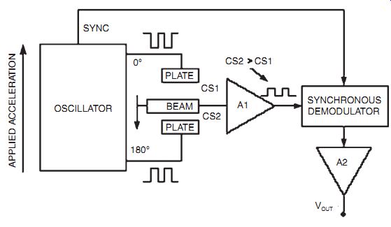
FIG. 3.20: ADXL-family accelerometers internal signal conditioning.

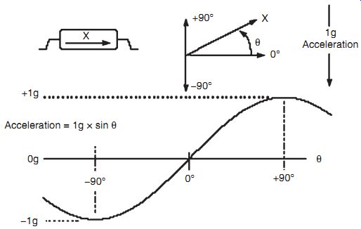
FIG. 3.21: Using an accelerometer to measure tilt.

The sensor's fixed capacitor plates are driven differentially by a 1 MHz square wave: the two square wave amplitudes are equal but are 180° out of phase. When at rest, the values of the two capacitors are the same, and therefore the voltage output at their electrical center (i.e., at the center plate attached to the movable beam) is zero. When the beam begins to move, a mismatch in the capacitance produces an output signal at the center plate. The output amplitude will increase with the acceleration experienced by the sensor. The center plate is buffered by A1 and applied to a synchronous demodulator. The direction of beam motion affects the phase of the signal, and synchronous demodulation is therefore used to extract the amplitude information. The synchronous demodulator output is amplified by A2 which supplies the acceleration output voltage, VOUT.

An interesting application of low-g accelerometers is measuring tilt. FIG. 3.21 shows the response of an accelerometer to tilt. The accelerometer output on the diagram has been normalized to 1g full-scale. The accelerometer output is proportional to the sine of the tilt angle with respect to the horizon. Note that maximum sensitivity occurs when the accelerometer axis is perpendicular to the acceleration. This scheme allows tilt angles from -90° to +90° (180° of rotation) to be measured. However, in order to measure a full 360° rotation, a dual-axis accelerometer must be used.

References

1. Herman Schaevitz, The Linear Variable Differential Transformer, Proceedings of the SASE, Volume IV, No. 2, 1946.

2. Dr. Ernest D.D. Schmidt, Linear Displacement - Linear Variable Differential Transformers - LVDTs, Schaevitz Sensors, http://www.schaevitz.com.

3. E-Series LVDT Data Sheet, Schaevitz Sensors, http://www.schaevitz.com.

Schaevitz Sensors is now a division of Lucas Control Systems, 1000 Lucas Way, Hampton, VA 23666.

4. Ramon Pallas-Areny and John G. Webster, Sensors and Signal Conditioning, John Wiley, New York, 1991.

5. Harry L. Trietley, Transducers in Mechanical and Electronic Design, Marcel Dekker, Inc., 1986.

6. AD598 and AD698 Data Sheet, Analog Devices, Inc., http://www.analog.com.

7. Bill Travis, Hall-Effect Sensor ICs Sport Magnetic Personalities, EDN, April 9, 1998, pp. 81-91.

8. AD22151 Data Sheet, Analog Devices, Inc., http://www.analog.com.

9. Dan Sheingold, Analog-Digital Conversion Handbook, Third Edition, Prentice-Hall, 1986.

10. F. P. Flett, Vector Control Using a Single Vector Rotation Semiconductor for Induction and Permanent Magnet Motors, PCIM Conference, Intelligent Motion, September 1992 Proceedings, available from Analog Devices.

11. F. P. Flett, Silicon Control Algorithms for Brushless Permanent Magnet Synchronous Machines, PCIM Conference, Intelligent Motion, June 1991 Proceedings, available from Analog Devices.

12. P.J.M. Coussens, et al, Three Phase Measurements with Vector Rotation Blocks in Mains and Motion Control, PCIM Conference, Intelligent Motion, April 1992 Proceedings, available from Analog Devices.

13. Dennis Fu, Digital to Synchro and Resolver Conversion with the AC Vector Processor AD2S100, available from Analog Devices.

14. Dennis Fu, Circuit Applications of the AD2S90 Resolver-to-Digital Converter, AN-230, Analog Devices.

Aengus Murray and P. Kettle, Towards a Single Chip DSP Based Motor Control Solution, Proceedings PCIM - Intelligent Motion, May 1996, Nurnberg Germany, pp. 315-326. Also available at http://www.analog.com.

16. D. J. Lucey, P. J. Roche, M. B. Harrington, and J. R. Scannell, Comparison of Various Space Vector Modulation Strategies, Proceedings Irish DSP and Control Colloquium, July 1994, Dublin, Ireland, pp. 169-175.

17. Niall Lyne, ADCs Lend Flexibility to Vector Motor Control Applications, Electronic Design, May 1, 1998, pp. 93-100.

18. Frank Goodenough, Airbags Boom when IC Accelerometer Sees 50g, Electronic Design, August 8, 1991.

4. Selecting Position and Displacement Transducers

As an application development manager for a position transducer supplier, I receive numerous queries on how to solve a broad range of position-measurement challenges.

These inquiries run the gamut from the common (aircraft flight-control surface movement) to the exotic (Formula One racecar suspension travel) to the seemingly impossible (three-dimensional tracking of a golf ball in flight from a fixed position).

These position-measurement challenges usually share one common element. They can be solved using a variety of solutions, but it's not always easy to determine the best one.

There are possibly more options for measuring position than any other type of sensed variable. While there may be more suppliers for pressure transducers, the variety of position transducer types and technologies is unmatched.

The 1997 Thomas Register lists 264 suppliers of pressure transducers and 229 suppliers of displacement and position transducers. However, there are 13 categories related to displacement and position measurement, compared to just four categories for pres sure measurement.

In this SECTION, I introduce you to various position-transducer selection parameters.

You'll also find information on position-measurement techniques, technologies, and choices.

Basic Terminology

A brief note on semantics: for ease of communication, this guide refers to transducers and sensors as being the same. While not strictly true, is generally irrelevant whether you are using a position sensor or transducer. The purpose of both is the same--to find out where something is! Transducers covered here provide position, displacement, and proximity measurements, which are defined as:

¦ position - location of the object's coordinates with respect to a selected reference

¦ displacement - movement from one position to another for a specific distance or angle

¦ proximity - a critical distance signaled by an on/off output

In this SECTION, I focus primarily on transducers for position and displacement measurement. Unless otherwise noted, I use the term "position transducer" to refer to displacement and proximity transducers as well.

The Parameters

On what basis should you select a position transducer? As a starting point, let's look at the laundry list of parameters shown in FIG. 4.1. While this list is not all-inclusive, it helps you begin to decide what parameters are relevant to your application.

Perhaps the first parameter to address in any application is whether the transducer can physically touch the object being monitored. If your application is sensitive to outside influences, a noncontact transducer may be the most appropriate. Otherwise, a contact sensor might offer advantages not found in a noncontact sensor.

FIG. 4.1: What are your requirements?

At first thought, noncontact transducers may seem like the superior solution for all applications. However, the decision isn't that clear cut. Noncontact products can emit potentially harmful laser- or ultrasonic-based signals. These products also rely on having a clear visual environment to operate in. Frequency response isn't always as high as with a contact sensor, but costs are often higher. Finally, operating-tempera ture ranges are typically not as broad.

Another parameter to consider early on is whether you need to measure linear or rotary movement. Note that using cable position transducers (like the one shown in FIG. 4.2), cams, pulleys, levers, electronics, software, and other methods can enable a rotary transducer to measure linear motion, and vice versa. Lack of space, cost, and ease of mounting are a few reasons for doing this.

Once you decide if you require a contact or noncontact solution and are measuring rotary or linear movement, selecting a transducer technology becomes much easier.

Next, determine if you're monitoring one-dimensional or multidimensional motion. If the motion is multidimensional, determine whether you need to measure in multiple dimensions or if the object is moving in multiple dimensions and you only have to measure one of them.

Often, multidimensional motion is measured with multiple one-dimensional transducers.

Also, think about the type of signal you need to obtain. If you need a signal that specifies a unique position, be sure to specify a transducer with absolute output. However, if all you need is relative position from a prior position or a simple on/off indicator, then incremental or threshold technology is more appropriate. FIG. 4.3 gives you a view of some incremental rotary optical encoders.

An important difference between incremental and absolute transducers is that incremental transducers typically need to be reinitialized after power-down by moving the monitored object to a home position at powerup. This limitation is unacceptable in some applications.

Threshold measurements are on/off in nature and usually involve limit switches or similar devices. As you might guess, absolute devices are usually more expensive than incremental or threshold devices.

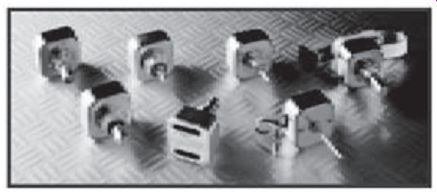
FIG. 4.3: Incremental rotary optical encoders provide quadrature digital output.

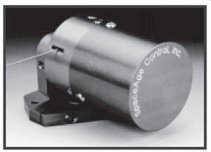
FIG. 4.2: Cable position transducers provide extended ranges in small sizes.

Travel, also known as range, varies from microns to hundreds of feet (or more, de pending on your definition of transducer). The range of many precision transducers is limited to 10 inches or less.

If your application needs to operate on the Space Station or some other size- and weight-sensitive platform, you need to specify the maximum values for the transducer's dimensions and weight.

The application's operating environment can have a large impact on your technology choice as well. You need to determine what operating and storage temperatures the device will be in and whether you need to meet commercial, industrial, or military environmental requirements.

Also consider whether excessive humidity, moisture, shock, vibration, or EMF will be encountered. Determine whether your environment has other unique aspects, such as high or low pressure or the presence of hazardous or corrosive chemicals.

An often-overlooked parameter is the method and time required for transducer installation and mounting. For testing applications, this parameter may not be so important. However, OEM and large-volume applications often require simple installation and removal to reduce labor costs and enable easy maintenance. See if the transducer can only be mounted with manufacturer-provided special mounting bases or if a variety of mounting techniques can be used. Besides the common threaded fastener approach, some other nonpermanent mounting techniques include suction cups, magnets, industrial adhesives, grooved fittings, and clamping.

In going through the previous parameters, you might have asked yourself, "Hey, what about accuracy?" While accuracy is certainly important and sometimes critical, it's often the last degree of freedom in the selection of a transducer. As you may know from experience, accuracy is not a well-agreed-on term. Typically, various components of accuracy, linearity, repeatability, resolution, and hysteresis are quoted for vendor convenience or per user requirements.

With the availability of software calibration tools today, linearity isn't as important as it once was. For many applications, in fact, repeatability is the most important component.

Accuracy is typically specified in absolute units like mils or microns or in relative units such as percent of full-scale measurement. If you are comparing the accuracy of one device against another, make sure you are comparing apples to apples. For example, see if the accuracies being quoted are at a single temperature or over a temperature range. If you need it, find out if temperature compensation is available.

If you expect to see significant numbers of cycles or if the transducer will be in ser vice for an extended period of time, specify the lifetime and reliability requirements as well. When choosing the transducer, find out what warranties are offered as well as how maintenance and repairs are handled.

A transducer that can be repaired in-house can reduce costs significantly. You should also consider what type of periodic recalibration is recommended and whether calibration procedures are provided.

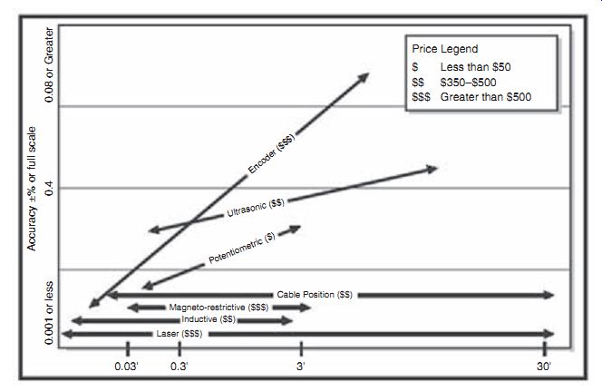
FIG. 4.4: Selection tradeoffs; typical performance of linear position transducers.

It's a good idea to ask vendors what type of use their transducers see most often.

Common uses include OEM, retrofit, industrial control, commercial, and test and measurement. Hopefully, the transducer has seen previous use in your type of application.

In the early stages of transducer specification, product cost sometimes doesn't even make the list. More often than not, this parameter gains importance as the project moves forward.

When determining costs, make sure to look at the initial acquisition cost as well as the cost over the product's life. For example, are special signal conditioning electronics, power supplies, electrical connectors, housings, installation tools, or mounting fixtures required? Ask the vendor for typical repair, maintenance, and replacement costs. And, inquire about the cost of the transducer in volume and single-unit quantities. The cost savings (e.g., a cost of $100 in volume but $600 in single quantities) may be an important factor if small-quantity replacement units will be needed in the future.

Another parameter that's occasionally overlooked is the time it takes the product to be delivered to you after you order it. The custom nature of some transducers combined with production processes and manufacturing economics requires lead times of eight weeks or more. This delivery schedule might be acceptable now, but what about in six months when you need extra quantities or a spare part? Evaluate whether or not you can afford to be without a part for an extended period of time.

Obviously, the transducer is going to be a part of a system. So, determine your preferred electrical input and output requirements. Common output choices include analog AC and DC voltage, resistive, current (4-20 mA), digital, and visual (meter).

Increasingly, outputs using sensor bus protocols are being offered. Most position transducers require 50 V or less, and some are self-powered.

Finally, for fast-moving applications, determine the maximum velocity or acceleration that needs to be monitored. Ensure that your data acquisition or control system has an adequate sampling rate to record the resulting data stream.

Check Your Requirements

Now that you're aware of the key parameters, you need to determine which ones are relevant to your application and of these relevant parameters, which are most critical.

If you don't prioritize your requirements, it's going to be difficult to make a selection decision. You may come to the conclusion that there is no transducer that can meet your needs. This may be true, but it's more likely that your requirements are too stringent and that you need to make a tradeoff to arrive at the optimum selection.

For example, an engineer recently approached our company looking for a transducer with ±0.0001 inch resolution over 30 inches, and he wanted to keep the cost under $500. He was adamant that all three specifications be met. Our products didn't meet all of his specifications, and we were at a loss as to where we would refer him. After some more discussion, we found out that the resolution requirement was only necessary over a limited portion of the total range and that the cost goal, while important, did have some flexibility.

Hence, in this situation, range was most important, followed by resolution, and then cost.

The moral of this story: focus on your top requirements. Make the best decision you can, given the specifications you need. And keep in mind that you can't have every thing, unfortunately.

Next Steps

In this SECTION, I've given you some parameters for selecting position transducers. But in case you hadn't noticed, I didn't provide any information on what type of technology you should select for your position transducer. The constant change in transducer technology and the difficulty in generalizing about a particular technology's capabilities and limitations mean there's no way I can cover this area in detail here. Refer to the previous sections of this SECTION for more details on various technologies.

Additionally, choosing the technology should come after determining and prioritizing your requirements. Once your requirements are well known, the choice of technology tends to be self-selecting.

For example, just knowing whether you require a contact or noncontact technology can cut your choices almost in half.

If you need the latter, a laser position sensor like the one in FIG. 4.5 may be a good choice.

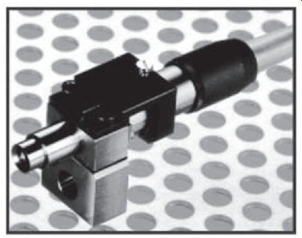
FIG. 4.5: Laser position sensors have resolutions of 0.1 µm or better.

To get a feel for the capabilities of some of the more prevalent linear position-measurement technologies, FIG. 4.4 maps out how these technologies compare against each other based on cost, accuracy, and maximum range. Note that not all technologies are shown.

It may be difficult to clearly define the parameter values you require as well as which parameters are most important in your application. However, it can be even more difficult to obtain these parameters from vendors and then compare one vendor's statements against another's. To get information on products beyond what you see in the vendor's product literature, review transducer-related publications such as Measurement and Control and Sensors for articles on position-measurement products and technologies. Also, be sure to ask your colleagues about their experiences and recommendations.

They may have a position transducer on hand that you may be able to test for your application.

Of course, in this day and age, make an effort to search Web engines and Internet newsgroups. Numerous engineering, instrumentation, and measurement-oriented newsgroups can be reached via search engines. Extensive sources of position-transducer manufacturers can be found in the Thomas Register and the Sensors Buyer's Guide.

Contact vendors and request references of similar applications. Ask these references why they selected the product they did and whether they're happy with their decision. Also, find out what other options they considered.

Finally, ask the vendor for product samples or evaluation units that you can use for testing before purchase. If the vendor is hesitant to do this, offer to provide them with a test report summarizing your evaluation. This information may be valuable to them, and they may be more willing to assist you.

NEXT: Pressure Sensors

PREV: Optical and Radiation Sensors

All related articles   Top of Page   Home