USING THE COUNTER-TIMER

Frequency Measurements

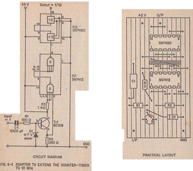
The highest frequency indicated by the counter-timer is 1 MHz. That is when the reading just exceeds 999.9 kHz and settles at 000.0 with the "Overspill" lamp lit. Of course the same indication will occur at 2 MHz, 3 MHz, etc. so that it is theoretically possible to determine with reasonable accuracy frequencies above 1 MHz provided that the order of the frequency being measured is known. The limiting factor, however, is the input stage gain which is virtually useless above 3 MHz.

The adaptor shown in Figure 6-1 enables frequencies between 1 MHz and 10 MHz to be measured with greater confidence.

It consists of an isolating capacitor C1, protection network R1 and D1 , and emitter-follower transistor feeding a double Schmitt-trigger in cascade. This is followed by a decade- counter which divides the input frequency by ten so that 9.999 MHz is presented to the counter-timer as 999.9 kHz.

It may be considered worthwhile to include this as an input stage in the main instrument, in which case suitable switching will have to be provided. Alternatively, if it is required to frequently monitor a high frequency oscillator say, the oscillator can have the adaptor built-in and connected to a suitable

"Frequency Check" terminal.

CIRCUIT DIAGRAM

FIG. 6-1. ADAPTOR TO EXT END THE COUNTER-TIMER TO 10 MHz PRACTICAL LAYOUT

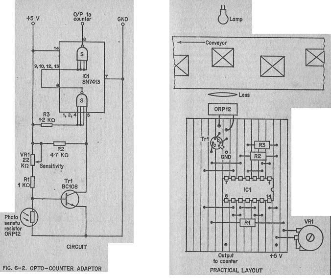
FIG. 6 - 2 . OPTO-COUNTER ADAPTOR PRACTICAL LAYOUT

Some of the more expensive communication receivers are fitted with digital tuning dials. Normally it is not practicable to directly measure signal frequency and so the counter is connected to the receiver local oscillator. This relates to the signal but with a displacement depending on the receiver i.f.

The problem may be overcome by starting the count, not from zero, but from a figure representative of either the i.f. or its complement, depending on whether the receiver local oscillator frequency is below or above that of the signal. Unfortunately, this technique is difficult to arrange with the counter-timer described in this guide..

A possible alternative to direct receiver frequency measurement is to use a digital heterodyne wavemeter. This simply consists of a stable oscillator connected to the counter, and tuned so as to "beat" with the received signal. The wavemeter frequency is measured, and hence, that of the signal. Care must be taken, however, to ensure that the measurement is not confused by harmonics, spurious beats from the receiver local oscillator and second channel detection. The method and its drawbacks can be demonstrated at low radio frequencies by using the pulse generator shown in Figure 4-5 as the heterodyne wavemeter.

A problem which does arise when measuring frequency relates to the signal waveshape and amplitude. Suppose, for example, that it is required to measure the frequency of ripple appearing on top of a low frequency pulse. Unless the ripple amplitude is comparatively large, the counter tends to measure the low frequency pulse only. One solution is to display the composite signal on an oscilloscope and use the counter-timer to measure the timebase frequency. The timebase period can then be related to the relevant part of the waveform with reasonable accuracy. Alternatively, a high-pass filter may be tried.

Pulse-Counter Unrelated To Time

Figure 6-2 illustrates a simple opto-electronic set-up for counting items on a conveyor belt. Other forms of transducers can be used for similar measurements. For instance, the number of revolutions made by a wheel can be determined from pulses produced by a microswitch operating from a simple cam. Sometimes it can be arranged that the wheel revolutions are related to distance so that the counter is actually displaying yards, meters, miles, etc. Usually it is necessary to clean up the pulses produced by mechanical transducers such as microswitches by using an anti-bounce circuit such as that shown in Figure 4-8.

Revs-Per-Minute

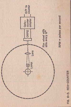
Figure 6-3

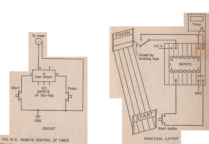
FIG. 6-4 . REMOTE CONTROL OF TIMER PRACTICAL LAYOUT

The techniques just described can be used to measure rpm by simply noting the number of pulses counted in one minute.

This can be tedious, and so another approach is to make the rotor produce 60 pulses during one revolution, when rpm also becomes pulses-per-second and can be measured as frequency.

This has the advantage of speeding up the measurement period so that the effect of any adjustment can be quickly noted. A suitable system is illustrated in Figure 6-3, with the photo-cell connected to an input circuit similar to that shown in Figure 6-2.

Timer Processes can be manually timed as follows:

1. Process starts ...... Press the "Reset" button.

2. Process completed. Press and hold down the

"Display-Hold" button and read the time.

Figure 6-4 illustrates a method of remotely controlling the timer. The J-K flip-flop is latched so as to hold the input "hi" and inhibit the timer. At this stage the counter is manually reset to zero. Timing is initiated by pressing S1. This latches the flip-flop "lo" until S2 is pressed, when the flip-flop latches "hi" and again inhibits the timer, allowing it to be read.

Similar methods to that just described can be used to measure very low frequencies and rpm. If the time taken for one complete cycle is measured in seconds:

Frequency (Hz) rpm Time (Secs) 60 Time (Secs)

The measurements just described require the timer to be manually reset to zero before making the next measurement.

A remote reset facility can easily be provided by simply fitting suitable terminals across the "Reset" button (S2 in Figure 5-1).

Some experimenters may wish to extend the timer facilities by providing two extra ranges. The unit as shown in Figure 5-1 uses switch-wafer S ic to select 10 Hz from pin 11 o f IC14 to provide 0.1S pulses. 15 pulses can be similarly obtained from pin 11 ofIC15, and 0.01S pulses from pin 14 o f IC14. In the latter case, it is desirable to arrange for switch-wafer S la to select decimal point dp3. Both new ranges will require switch- wafer Sib to ground pin 5 of IC10 and pin 8 of IC16. The maximum display reading for each range will then be:- 99.99 Seconds in 0.01S increments 999.9 Seconds in 0.1S increments 9999 Seconds in 15 increments.

Analog-To-Digital Converters

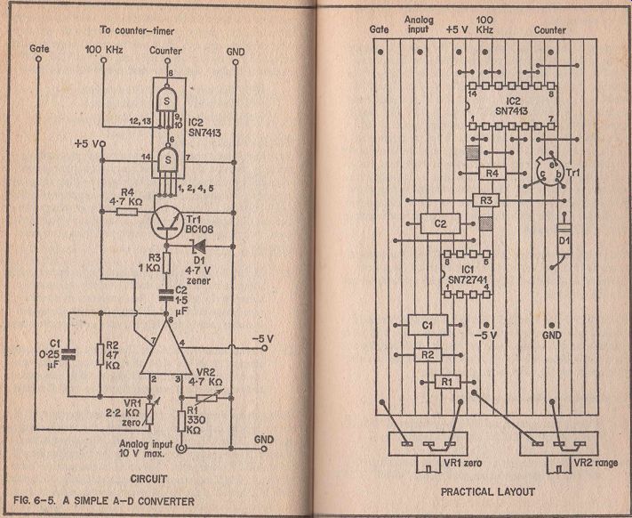
FIG. 6-5 . A SIMPLE A - D CONVERTER

Basic digital instruments are counters which can easily be made to measure time and frequency because these are electrically processed in precise increments. Other parameters are not so convenient and normally require an analog-to-digital (A/D) converter. The analog input is usually in voltage form, because this is readily derived from quantities such as resistance, current and power. AD converters fall into two main groups:-

1. Digital Bridge: Voltage produced by the instrument is adjusted incrementally until it exactly balances the voltage to be measured. The increments relate directly to a binary code which is applied to the display via decoders such as the SN74141 used in the counter-timer.

2. Proportionate Clock Gate: The voltage to be measured is arranged to set the width of a gate pulse. This in turn controls the number of clock pulses fed to the counter, so that pulse count is proportionate to applied voltage.

Although the design of a comprehensive and accurate A/D converter is outside the scope of this guide, the simple circuit shown in Figure 6-5 may be of interest. Fitted to the timer- counter it will produce a two digit display indicating 0 to +5 volts in 0.1V increments. This could be increased to three digits and 0.01 V increments by injecting 100 kHz clock-pulses into IC2 instead of the 10 kHz shown, but then the decimal point would be in the wrong place. In any case, the linearity and accuracy of the circuit are not compatible with three figure resolution.

To operate, the counter is switched to the highest frequency range so that a 10 mS gate pulse is available to the inverted input of IC1 via VR1. Here, the pulse is integrated by C1l to produce the wedged shaped pulse illustrated in Figure 6-5 ' insert, and then fed via TR1 inverter, and D1 protection and dc restorer, to the first Schmitt-trigger in IC2. The analog input voltage applied to the non-inverting input of IC1 effectively sets the wedge amplitude. When the input is low, only the narrow part of the wedge projects above the Schmitt threshold potential to produce a narrow output pulse, but as the analog input is increased, so does the wedge amplitude and output pulse width. The output pulse fed to the second Schmitt-trigger in IC2 is used to gate the 10 kHz clock-pulses, causing the number fed to the counter to be proportionate to the analog input voltage.

The 10 kHz clock-pulses may be derived from the counter-timer if it is fitted with the crystal controlled frequency reference illustrated in Figure 4-6; otherwise a separate source 'must be provided.' The SN72741 is a Standard operational amplifier which is obtainable in several styles as shown in Figure 6-5. It requires a negative as well as positive power supply. Both supplies can be obtained from two 4.5 volt batteries connected hi series with the center tap taken to the ground rail.

The converter is calibrated as follows:

1. With no analog input, set VR1 for a display of "000.1", then back off so that the display just reads zero.

2. With a known analog input voltage not exceeding +5V, set VR2 for the appropriate reading, e.g. "004.5" (4.5V).

Index | Prev. |