AMAZON multi-meters discounts AMAZON oscilloscope discounts
.
In some cases, you can diagnose a problem simply by examining the symptoms logically. More often, however, any given symptom or set of symptoms indicates several possible faults. The service technician depends on his test equipment. Although certainly some technicians are better than others, to an extent no technician is better than his or her test equipment. The best technician in the world would be severely limited with inadequate test equipment.
Various common types of test equipment are mentioned throughout this guide. In this section, we specifically focus on several different types of test equipment, emphasizing fairly recent devices as much as possible.
The first requirement for a well-equipped electronics work bench is a large work surface. You might find yourself with several pieces of equipment opened up and spread out at the same time, plus you need room for any test equipment. Therefore, your work surface should be as large as possible.
Adequate lighting is an absolute must. A dimly lit work area will slow you down and increase the chance of errors. Use multiple light sources so you can’t block off the light with your own body or a piece of equipment.
A high-intensity lamp on a flexible goose-neck, as illustrated in -- Fig. 1, can be an extremely handy item to have— you can focus the light wherever you need it. A lot of equipment has dark nooks and crannies you need to see into.
Your work area should have several electrical outlets. You can never have too many. There always seems to be one more thing you need to plug in. Avoid using cube taps and extension cords as much as possible because they can be fire hazards if overloaded. Many distributors sell power strips, which are convenient and safe (-- Fig. 2). Many even have built-in surge protectors. Most have a handy master power switch that is useful in some circumstances. It’s also a good way to ensure everything is off when you close up for the night.
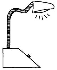
-- Fig. 1 A high-intensity lamp with a flexible goose neck is a useful item
on the workbench.
What test equipment will you need? It depends on just what type of work you do. A multimeter (VOM or VTVM) is absolutely essential for electronics workbenches. If possible, you should have at least one VOM and one VTVM. The multimeter is the technician’s right arm.
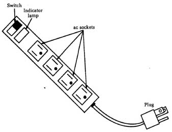
-- Fig. 2 A power strip safely provides extra ac outlets. Switch; Indicator
lamp; Plug.
The technician’s left arm is the oscilloscope, another essential device for virtually’ all electronic workbenches. Anytime you are dealing with an ac signal, a scope is useful because it permits you to actually see the waveform. You also can measure the volt age at any point in the cycle, check for distortion, measure the cycle period, and make many other tests.
The multimeter and the oscilloscope are standard items used in all types of electronics work. Other generally useful devices include variable power supplies, Variacs, and signal generators. There are many different types of signal generators for various applications; several common types are discussed in this section. Other devices include capacitance meters, frequency counters, specialized signal generators, and signal tracers.
Don’t scrimp on your test equipment. Your accuracy will be no better than the capabilities of your equipment. Don’t over spend on features you don’t need or on equipment you will rarely, if ever, use. Make sure, however, that you do get what you need. Nothing is worse than being stumped on a servicing job because you don’t have the right equipment. Occasionally, this situation is inevitable because you will undoubtedly run into something outside your usual area. If insufficient equipment problems plague you frequently, however, you need to be better prepared.
Multimeters
A multimeter measures various electrical parameters—usually voltage, current, and resistance. Multimeters are used in many of the test procedures in this guide, especially in sections 2 and 4.
A VOM (volt-ohm-milliammeter) is a passive device. It does not include an active amplifier or buffer stage, so the input impedance (resistance) is fairly low. Some cheap VOMs have input impedances as low as 1,000 ohms per volt. Such units are virtually useless for practical electronics work because they can excessively load down the circuit being tested, throwing off the measurement.
The unofficial standard for professional VOMs has long been considered 20,000 per volt. Modern, high-quality VOMs usually have input impedances of 50,000 or 100,000 ohms per volt.
VOMs are usually lightweight and portable. Most VOMs have a small internal battery for the ohmmeter section, which means you don’t have to be tied to a power source.
A much higher meter impedance is necessary for some precision measurements. In this case, use a multimeter with an active amplifier/buffer stage. In the past, the amplifier was a tube circuit, so this type of device traditionally has been known as a vacuum tube voltmeter (VTVM). Today, of course, tubes are increasingly scarce. Even when such a device uses only semiconductor components, it’s still often called a VTVM. A better name might be electronic multimeter (EMM).
VTVMs, or EMMs, have high input impedances, typically 1 M-ohm per volt. They are very precise, but tend to be more expensive and bulkier than VOMs. Also, a VTVM or EMM, being an active device, requires some sort of power supply.
Today, the trend is toward digital. Digital multimeters, or DMMs, are extremely popular. Many are as small and portable as a VOM. Often, they are powered from a small internal battery (9-volt transistor radio batteries are often used). A DMM usually has an input impedance comparable to a VTVM, but it also offers the convenience of a lightweight VOM.
Digital multimeters offer a number of significant advantages over their analog counterparts. They are easier to read without ambiguity. A display reading of 7.83 volts (V) is quite unmistakable and precise. On an analog VOM, you must approximate the value from the position of the meter’s pointer between standardized mark-points. It also can be difficult to determine exactly where the pointer actually is in relation to the meter’s scale face, especially if viewed from any angle other than straight head-on. Parallax errors are practically inevitable when you are using an analog meter. Parallax errors are not a problem with a DMM, regardless of the viewing angle. Either you can read the displayed numbers or you can’t. If you look at a DMM from a bad angle, you are not going to mistake a reading of 7.83 for 7.69 or 8.12.
Another advantage of DMMs is their high input impedances, typically at least 1 M-ohm (1,000,000 ohm) per volt. A high input impedance translates to high accuracy and sensitivity. In an analog VOM, the input impedance is usually much lower. For a long time, 20 k (20,000 ohm) was considered standard, although many 50k-ohm (50,000 ohm) and look-ohm (100,000 ohm) VOMs are available. A VOM with a FF1’ input stage, or a VTVM, generally has a higher input impedance than a standard VOM. Some inexpensive VOMs have input impedances as low as 2 k-ohm (2,000 ohm) per volt. Such units are not suitable for serious electronics work.
The importance of a high input impedance for a voltmeter is illustrated in Fig. 3. The voltmeter measures the voltage drop across some resistive element in the circuit, but the internal resistance (impedance) of the voltmeter itself is in parallel with the intended circuit resistance. This situation can affect the resulting reading, often to a surprising degree.
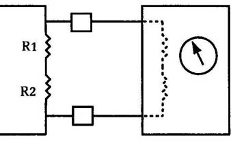
-- Fig. 3 The input impedance of a voltmeter acts like a parallel resistance
across the circuit under test, affecting the reading.
Let’s assume we are feeding 9 V through two resistors, as shown in the diagram. Resistor R1 had a value of 25 k-ohm (25,000 ohm) and resistor R2’s value is 50 k-ohm (50,000 ohm. The total series resistance is simply the sum of the two component resistances.
Rt = R1+ R2
= 25,000 + 50,000
= 75,000 ohm
= 75 k
The current flow through the resistors can be found with Ohm’s law:
I = E/R
9/75,000
=0.00012 A
= 0.12 mA
The same amount of current flows through each resistor in series, so the voltage drop across an individual resistor (R^2, in our example) can be found be rearranging the Ohm’s law equation.
E = IR
= 0.00012 X 50,000 =6V
This is all quite simple and straightforward. When you try to actually measure this voltage drop, however, the input impedance of the multimeter is added in parallel with resistor R2. The effective total resistance in the circuit becomes equal to:
[…]
Consider what happens if you use a cheap VOM with an input impedance of just 2k-ohm (2,000 Ohm). The circuit’s total effective resistance becomes equal to:
= 25,000 + 1,923 =26,923 L
Therefore, the current flow through the circuit is changed to:
= 0.00033 A
= 0.33 mA
So the voltage drop we read across resistor R is:
E = IR
= 0.0003 3 x 1923
=0.54 V
That is ridiculously off from the expected 6 V we should get. Conditions improve if a VOM with an input impedance of 50 k-ohm (50,000 ohm) is used.
= 0.00018 X 25,000 = 4.5 V
…better, but it’s still hardly an accurate voltage reading.
Now, let’s see what sort of reading we’ll get with a DMM that has an input impedance of 1 M-ohm:
72,619 Ohm
= 0.00012 A
= 0.12 mA
= 0.00012 x 47,619 = 5.4 V
This is reasonably close with the DMM, especially compared to our earlier examples. Actually, this is very much a worse-case scenario, and you usually won’t run across such extreme errors in practical electronic work.
The input impedance of a multimeter is not fixed. Instead, it’s so many ohms-per-volt. The input impedance is multiplied by the range setting. For instance, if you were using a 10 V setting on each of the multimeters in this example, the impedance of the 2 k-ohm VOM would be more like 20 k. Similarly, the 50 k-ohm VOM would have a practical input impedance of about 500k-ohm on this range, and the 1 ML DMM would have an effective input impedance of about 10 M-ohm).
Digital multimeters usually offer a number of extra functions not available on most analog multimeters. These features aren’t essential, but they can be nice to have and don’t add appreciably to the overall cost. A conductivity test function seems to be quite common on modern DMMs. Conductivity is simply the reciprocal of resistance:
Conductivity = 1 / Resistance
Conductivity is measured in units called mhos. Of course, mho is simply ohm backwards. Conductivity measurements are useful for very low resistances. For example, 22,500 mhos is a lot more convenient value than 0.0000444 Ohm. In practical electronics work, however, the conductivity test function is of very limited practical value. It’s certainly not a feature that most electronics technicians should want to pay extra for. Today, electronics technicians use the unit Siemens, instead of mhos.
DMMs also often include functions for measuring such electrical parameters as capacitance and frequency, as well as specialized diode and transistor testing. Until recently, digital multimeters were considerably more expensive than their analog equivalents, but now a good DMM can be purchased for under $50. I’ve seen some in the $20 to $30 range.
The analog multimeter is, however, far from obsolete. For some testing procedures, an “old-fashioned” VOM will do a lot better job than an up-to-date model DMM. For many electronic tests, the exact, multi-digit precision of a DMM isn’t really needed. For example, it probably doesn’t matter too much if a circuit’s power supply is putting out 9.12 V or 8.93 V, instead of exactly 9.00 V.
In many practical testing procedures, the exact measured value isn’t as significant as the amount of change in the value over a short period of time. An analog VOM would certainly be a better choice than a DMM for such applications.
An example of this type of test would be the use of an ohm meter to test a capacitor. (Refer to section 4.) Essentially, when the ohmmeter’s test voltage is first applied across the capacitor’s leads, the pointer should jump to a very low value, then slowly move back to a higher resistance value as the capacitor is charged. This process is very clearly visible on an analog meter, but on a DMM, the result would be just a blur of numbers changing too rapidly to be read. The test would be meaningless on a DMM.
Ideally, if you do more than casual work in electronics, you should own both a digital multimeter and an analog multimeter. Although there is considerable overlap in their functions, they are each often good for different purposes. If you can’t afford both, we recommend that you go with an analog VOM or FET voltmeter first. The DMM can wait until you can afford it. Generally speaking, an analog multimeter will tend to be more versatile. If you are working seriously enough in electronics to require the precision of a digital readout, you definitely should invest in a simple analog VOM as a backup. It won’t go to waste.
This is not to say that any electronics technician wouldn’t find real advantages in having a DMM handy, but the advantages tend to be in the realm of luxuries, rather than absolute necessities. There is a tendency today, fostered by advertisers, that digital is automatically better for everything, and that isn’t true.
Even if you primarily service digital circuitry, an analog VOM would still be the better choice if you had to restrict yourself to just a single multimeter. Fortunately, prices have come down sufficiently that few of us really have to make an either/or choice. It’s not all that expensive to buy both an analog VOM and a DMM.
Digital circuitry is great, but it’s important to keep things in perspective. There is no reason to throw out all analog circuitry and devices. In fact, there are often good reasons not to do so. Analog is better for some things than digital, just as digital is better for other purposes. It makes good sense to use both technologies, choosing the one most appropriate to the specific task at hand.
A well-stocked electronics workbench should have at least an analog VOM and a DMM. An analog VTVM or EMM would also be very desirable. If you can afford it, it’s often useful to have several VOMs with spring-loaded clip leads. You can then monitor different parts of a circuit simultaneously.
Adapters for multimeters
The standard multimeter measures volts, ohms, and milliamperes, so it’s quite a versatile device. It can be made even more versatile with special add-on adapters to permit additional types of measurements. Usually these adapters convert some other parameter into a proportional voltage.
These adapters need not be particularly complex. For example, an ordinary semiconductor diode can be used as a simple temperature-to-voltage converter. The scale won’t be linear over a very wide range, but in some applications, it’s sufficient.
A number of multimeter adapters are available commercially, especially from manufacturers of DMMs. Usually, how ever, you have to build one yourself. Plans can be found for these adapters in the popular electronics magazines (Radio Electronics, Modern Electronics, Hands-On Electronics, etc.).
Typical multimeter adapters create a proportional dc voltage from such parameters as:
• temperature
• capacitance
• frequency
• light intensity
Other adapters extend the range of the multimeter, permitting you to read very large or very small voltages and/or currents. Adapters are also available to accurately measure ac voltages above the basic line frequency (60 Hz). For example, the circuit shown in -- Fig. 4 converts an ac voltage in the rf range into a proportionate dc voltage. Adapters for measuring true root- mean-square (rms) values by converting them to a proportionate dc voltage are discussed in section 8.
R1 --- 10k-ohm Trim pot (Calibrate—adjust for approximately 6.5k-ohm )
R2 --- 47k-ohm Resistor
C1 --- 0.82 uF Capacitor
C2 --- 120 pF Capacitor
D1, D2 --- Small signal diodes
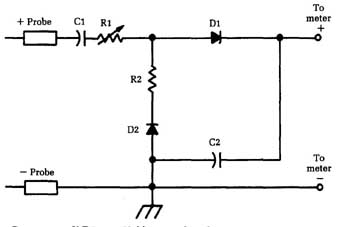
-- Fig. 4 This circuit converts an ac voltage in the RF range to a proportion
ate dc voltage.
Oscilloscopes
Probably the most important and useful piece of electronic test equipment is the multimeter, but the oscilloscope runs a very close second. It’s particularly helpful when dealing with signals that change over time. You can use an oscilloscope to measure dc voltages, but this method will usually be technological overkill. A multimeter (either digital or analog) almost certainly would be more convenient for the job. When it comes to ac signals, how ever, the oscilloscope wins hands down over the multimeter.
Most multimeters, if they can measure ac voltages at all, can give an accurate reading only if the signal in question is a relatively pure sine wave, with no harmonic content or other over tones. A more complex waveform will tend to confuse the meter because an ac voltage is not a straight-forward value like a dc volt age. For example, 3 volts dc (Vdc) is 3 volts dc, and that is that, but an ac voltage, by definition, changes values continuously over time in a repeating pattern. A 3.0 volt ac (Vac) signal will probably have instantaneous values like 2.3 V, 0 V, — 0.7 V, or even 4.1 V, depending on what point in the cycle you are measuring.
Sometimes an ac voltage is measured as a peak value, the maximum instantaneous voltage the waveform ever achieves during its cycle (-- Fig. 5). Notice there are two peak voltages: a positive peak voltage, and a negative peak voltage. Assuming the waveform is symmetrical around true zero (ground potential), these two peak voltages will be equal, except for their opposing polarities. The peak voltage of an ac waveform can be useful in determining whether the maximum ratings of sensitive components are ever exceeded, but it doesn’t really tell much about the waveform signal itself. In addition, it would be very difficult to design a circuit that would display the peak voltage value on an analog meter or a digital read-out.
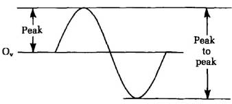
-- Fig. 5 The peak voltage is the maximum instantaneous voltage occurring
during the waveform’s cycle.
Often, an ac waveform won’t be symmetrical around true zero. That is, a given waveform might have a positive peak voltage of 4.2 V and a negative peak voltage of — 1.8 V. Just saying the peak voltage of the waveform is 4.2 V would be quite misleading for most purposes. A peak to peak voltage will, at least, give more of an idea of the waveform’s magnitude. The peak to peak voltage is simply equal to the difference between the positive and negative peak voltages:
E_PP = Ep+ — Ep-.
…where is the peak to peak voltage, E_p+ is the positive peak volt age, and E_p- is the negative peak voltage.
Four our example waveform with a positive peak voltage of 4.2 V and a negative peak voltage of—1.8 V, the peak to peak volt age is equal to:
= 4.2 — (—1.8)
= 4.2 + 1.8
= 6.0 V, peak to peak
Unfortunately, the peak to peak voltage still doesn’t tell very much about how the ac signal will function in a given circuit. Standard formulae, such as Ohm’s law, won’t work. Part of the problem is that , for most ac waveforms, the peak voltages occur for only a very brief portion of each cycle. (There are exceptions, of course. A square wave is at its positive peak voltage for half of each cycle, and at its negative peak voltage the rest of the time.)
To get a meaningful ac voltage value for the waveform as a whole, it’s generally necessary to take some sort of average. Several instantaneous voltages per cycle are added together and the sum is divided by the number of samples. Unfortunately , for a symmetrical waveform, the complete average will always work out to 0 (plus or minus minor rounding off errors). Obviously, this value is utterly useless. An average voltage is therefore normally taken over just one half of each waveform. For a sine wave, the average voltage always works out to 0.636 times the peak voltage. Other waveforms will have different average values.
Even with the average voltage, Ohm’s law and other important electronics formulae still don’t work. Moreover, it requires some complicated circuitry to measure average ac voltages.
For most practical purposes, ac values are given in root- mean-square (rms). Such values are calculated through some rather complex mathematics. For sine waves (but no other waveforms) the rms value equals 1.11 times the average, or 0.707 times the peak. Peak, average, and rms values are compared in Table 1.
The big advantage of rms values is that they allow us to use Ohm’s law and other common equations just as we would in a dc circuit. According to Ohm’s law, the current flow is equal to the voltage divided by the resistance. A rms ac voltage will give the same current value as the comparable dc voltage. For example, let’s say we have 10 Vdc being dropped across a 250 resistance.
Table 1 AC voltages can be measured as peak, average, or rms values.
=, Peak, Peak to peak, Average, RMS
[Find the known value unit in the top line. Follow the column down until it intersects the line for the desired value unit. Multiply by the constant in the space. For example, if you know the average value and want to find the rms value, multiply the average value by 1.11.]
The dc current is therefore equal to:
I=E/R
=10/250
= 0.04 A
If we replace the 10 Vdc with a sine wave of 10 V rms through the same 250 resistance, we will also get an ac current value of 0.04 A rms. However, the average voltage for that same ac signal would be about 9 V, and the peak value would be 14.1 V, resulting in rather meaningless current values if we try to use Ohm’s law.
It’s relatively easy to design an ac voltmeter to measure the rms values of sine waves, but such a meter won’t be able to give accurate readings for any other waveform, such as a triangle wave or a square wave. Even worse, the ac voltmeter won’t give you any indication of whether the signal being monitored is reason ably close to a sine wave or not. It just assumes the input signal is in the form of a sine wave and measures it accordingly. Clearly, this method will give some totally meaningless readings for certain waveforms.
With an oscilloscope, notice the actual waveform. You can easily see the peak points and its zero lines. Notice whether or not the waveform is symmetrical. If the ac waveform is riding on a dc voltage, this is also clearly visible. An oscilloscope permits you to actually see the signal being monitored, by drawing a picture of it on a CRT screen (similar to that of a television set.) The oscilloscope, therefore, permits us to perform many test procedures that would be impossible or impractical with a multi meter. Section 5 covers a number of common test procedures using the oscilloscope.
Like most other types of electronic equipment, oscilloscopes range from relatively simple to very complex devices. They are available with numerous specialized features, which might or might not be useful in the specific type of electronics work you do.
A simple, basic oscilloscope displays one waveform at a time, which is useful for many purposes, but sometimes it’s not enough. You cannot compare phase relationships (timing of cycles) among various parts of the circuitry. It would also be difficult to determine whether a particular stage was adding subtle distortion (mishaping of the waveform) of an input signal. Under such conditions, a dual-trace oscilloscope is needed.
Dual-trace oscilloscopes
A dual-trace oscilloscope, sometimes called a dual oscilloscope, is essentially two oscilloscopes in one. As the name suggests, two signal traces are displayed on the CRT screen, which is very useful for troubleshooting and servicing. Two signals can be com pared directly. For example, you can monitor the input signal for a questionable stage and its output simultaneously, making it relatively easy to see if the stage in question is doing what it’s sup posed to do to the signal or if it’s distorting or shifting the signal in some unintended way. In many electronic circuits, signal phase is crucial.
How can you find an out-of-phase signal with a single-trace oscilloscope? Phase is the description of the signal timing—when each cycle begins and ends — as compared to some reference. It’s a comparative, rather than an absolute, parameter (such as volt age or resistance). A dual-trace oscilloscope permits you to make such comparisons.
The obvious way to design a dual-trace oscilloscope would be to build a CRT with two independent electron guns, each with its own set of deflector plates—in other words, two CRT tubes in a single glass envelope. Unfortunately, this approach can be very expensive, although it’s used in some high-end dual oscilloscopes. Two CRT tubes also introduces a number of tricky design problems, such as how to keep the beam from one electron gun from being affected by the deflector plates of the other gun. It can be done, but it’s not easy or inexpensive.
Most practical dual-trace oscilloscopes use some type of digital switching to simulate the effect of two electron beams, even though only a standard single-gun CRT is used. There are two basic ways this switching is done: alternate mode and chopped mode. Most dual-trace oscilloscopes can operate in either switching mode, depending on the sensed signals and/or the front panel control settings. A simplified block diagram of a dual-trace oscilloscope is shown in -- Fig. 6. The difference between the two modes is in how the electronic switch is operated.
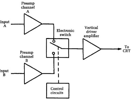
-- Fig. 6 A dual-trace oscilloscope switches back and forth between two input
signals. Preamp channel; Input A; Input B; Vertical driver amplifier; Electronic
switch; To CRT
In the alternate mode, trace A is first drawn for one complete sweep cycle. That is, the beam is moved across the screen, just as in a regular, single-trace oscilloscope, but at the end of the sweep cycle, when the beam reaches the far end of the screen, input A is switched out and input B is switched in. An offset voltage moves the center (zero) line of this second trace, so the two traces don’t overlap (unless you choose to set the controls for such overlap , for certain test functions). Now, trace B is drawn across the screen for one complete sweep cycle. When the beam reaches the far end of the screen, the input is switched back to signal A, and this trace is redrawn for the next sweep cycle. The oscilloscope’s CRT screen is coated with a phosphorous with some delay. This coating, coupled with persistence of vision, makes it appear that both traces are being continuously displayed, unless the sweep frequency is very low.
The chopped mode is rather similar, except that the switching takes place much more frequently. It does not wait until the end of a sweep cycle; instead, the beam is switched back and forth between the two traces many times during each sweep cycle. A little bit of trace A is drawn, then signal A is turned off and a little bit of trace B is drawn. If an appropriate switching rate is used, the two traces will appear to be continuous lines, but they actually will be broken up, as illustrated in exaggerated fashion in -- Fig. 7. These breaks in the traces might become visible at some frequencies.
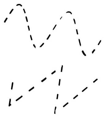
-- Fig. 7 In the chopped mode, the oscilloscope switches between the two signals
many times per sweep cycle.
For some signal pairs, the alternate mode will work better and provide more precise information about the signals. In other cases, the chopped mode is the better choice. Actually , for most noncritical work, the choice of mode probably won’t matter too much—either will work fine.
Dual-trace scopes are now the norm, except for small portable scopes and very inexpensive bench scopes. Single-trace scopes are still manufactured and used, but they are becoming increasingly rare. In the future, there will be even more extensive multiple-image scopes.
Storage oscilloscopes
Occasionally, while working on an electronic circuit, a technician might want to study certain displayed waveforms for awhile. With a continuous, unvarying periodic (ac) waveform, this is no problem, since the pattern is repeatedly redrawn during each cycle of the oscilloscope’s sweep signal. One-shot signals, how ever, such as those used in switching circuits, come and go quickly. Often the entire signal of interest lasts only for a few milliseconds, and then it’s gone, leaving just a flat trace on the oscilloscope’s screen.
The persistence of the phosphors coating the inner surface of the oscilloscope’s CRT screen permit them to glow long enough for the trace to be seen, but the displayed trace fades away within seconds. This often might not be long enough for the technician to read enough information from the displayed waveform. Obviously, this type of problem becomes more crucial as the signal increases in complexity and detail.
The solution to such problems is to use a special type of oscilloscope known as the storage oscilloscope. A storage oscilloscope can be used as a regular oscilloscope, duplicating all the standard functions, but it also features a special storage mode to permit relatively long-term display of nonperiodic (not repeating) signals. To accomplish this long-term display, the storage oscilloscope uses a special type of CRT. The basic structure of this device is illustrated, in somewhat simplified form, in -- Fig. 8.
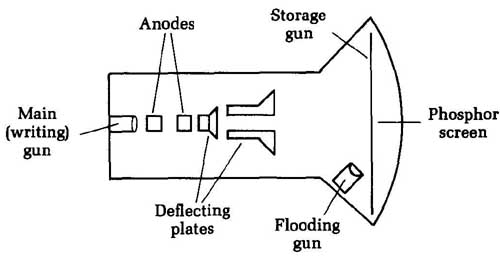
-- Fig. 8 A storage oscilloscope uses a special type of CRT with two electron
guns and a storage grid just inside the display screen. Anodes; Storage gun;
Main(writing) gun ; Phosphor screen; Flooding gun.
This type of storage CRT and the simpler CRT used in most basic oscilloscopes differ in two main respects. In the storage oscilloscope, the CRT has two electron guns, instead of just the usual one, and a storage grid of tiny electrodes mounted just in side the phosphor-coated display screen. The two electron guns in the storage oscilloscope’s CRT are called the main gun and the flooding gun.
The main gun functions just like the electron gun in an ordinary CRT. It produces the electron beam that draws the actual signal trace on the display screen. In the basic (nonstorage) mode, the flooding gun and the storage grid are left unused.
When the oscilloscope’s storage mode is activated, the electrodes in the storage grid are saturated with a negative electrical charge just before the momentary signal trace is drawn on the display screen by the main gun. The electrodes that are struck by the directed electron beam from the main gun as it draws the trace take on a localized positive charge. The other electrodes in the storage grid, which are not touched by the main gun’s electron beam, don’t pick up a positive charge. When the complete de sired waveform appears on the face of the CRT, the saturating negative charge is removed from the storage grid. The storage grid is specifically designed so that the positive charge on individual electrodes decays at a very slow rate, unless it’s deliberately re moved by re-saturating the entire grid with an external negative charge.
The flooding gun now takes over, irradiating the entire storage grid, which prevents the electrons from the flooding gun from reaching the phosphor-coated screen, except in those areas holding a localized positive charge. As a result, the original waveform trace continues to be displayed on the oscilloscope’s screen. As the glowing phosphors start to fade, they are continuously re energized by new electrons from the flooding gun.
The stored signal can be held and displayed, usually up to a maximum of several minutes. Infinite storage times are not possible, of course, because the storage grid electrodes cannot hold their charge indefinitely. The stored charge inevitably leaks off within a few minutes. Even so, the stored waveform is held long enough for the technician to examine it quite thoroughly.
Not surprisingly, storage oscilloscopes are considerably more expensive than standard oscilloscopes. If you need the storage function, however, the increase in price is well worth it.
Digital oscilloscopes
There is no question that the big trend in electronics over the last decade or so has been the general move from analog to digital circuitry. It should not be at all surprising that a number of digital oscilloscopes are now available.
Unlike the digital multimeters discussed earlier, the final output of a digital oscilloscope is still in analog form—the wave-shape is visually drawn, not represented by displayed numerical values. The difference is in how this is done. A digital oscilloscope uses digital circuitry to prepare the signal for display. In a digital oscilloscope, the analog signal to be monitored is converted into digital form for processing and multiplexing, then it’s converted back into an analog image for the final display.
Some digital oscilloscopes don’t even have a CRT. A multiplexed arrangement of light-emitting diodes (LEDs) often is used to display the waveform. By lighting up only the appropriate LEDs in the matrix, it’s possible to draw the waveform in dot-to-dot fashion. Obviously, the more LEDs there are in the matrix, the clearer the image will be and the more detail will be possible.
More recently, liquid crystal displays (LCDs) have been used for this purpose, permitting lower power consumption, simpler multiplexing circuitry, and less expensive construction (each individual LED has to be soldered into the circuit). The display signal data must be in digital form to light up the appropriate LED or activate the appropriate spot on a LCD in a display matrix.
An LED display tends to offer a little less detail than a CRT, but it’s less bulky and less fragile. It also does not require the high operating voltages a standard CRT demands. A LCD display can be even smaller and consume even less power than an LED display. Hand-held dual-trace oscilloscopes are available with LCD displays. A hand-held unit would not be practical using a standard CRT.
Unlike analog and digital multimeters, there would be no particular advantage for most technicians to own both an analog oscilloscope and a digital oscilloscope. They both perform essentially the same functions, just using different circuitry.
A special type of digital oscilloscope may use either a CRT or an LED/LCD display, but the digital circuitry is employed for signal processing purposes. The digital storage oscilloscope (DSO) is becoming increasingly popular among serious electronics technicians; however, the cost and expense of such instruments place them outside the reach of most electronics hobbyists.
The DSO takes the idea of the analog storage oscilloscope one step further. In an analog storage oscilloscope, the stored signal will fade away after a few minutes. A DSO, on the other hand, can hold the displayed signal indefinitely, as long as power is continuously supplied to the instrument. The data about the displayed signal is stored in numerical form in a digital memory, not just in electrical charges within the display screen. If a DSO is combined with a computer, as is often done, the signal can even be recorded for permanent storage and later recall and reuse.
Because the stored signal is in digital form, it can be manipulated in a number of ways. For example, certain features of the displayed waveform can be highlighted for emphasis, or the technician can enlarge the display to “zoom in” on areas of particular interest. The stored signal can be combined or compared with some other reference signal stored at an earlier time. Another ad vantage of the DSO is that, as a rule, digital timing can be more accurate than analog timing.
When shopping for a digital storage oscilloscope, all other factors being equal, choose the DSO with the longest record length specification. The record length determines how long the stored waveform can be; that is, how much information the DSO can hold at a time.
In addition to the analog bandwidth specification (which is essentially the same for both digital and analog oscilloscopes), you will also need to consider the sampling rate. The analog input signals are converted into digital form by sampling their instantaneous voltages many times per second. The speed at which this is done is called the sampling rate, and the faster the better. The sampling rate is usually given in the form of the highest usable signal frequency for the DSO’s maximum sampling rate.
According to the Nyquist theorem, the sampling rate must be at least twice the frequency of the signal to be digitized, or a form of distortion known as aliasing will occur. This distortion disguises the signal frequency and gives totally meaningless results.
If the sampling rate is just twice the signal frequency, the signal’s frequency can be measured accurately, but all details of the actual waveshape will be lost. For this reason, some manufacturers of DSOs specify the sampling rate for four or more points per cycle or period. Before comparing sampling rate specifications for competing DSOs, make sure you know how the figure was de rived. The four-points system will give less impressive numbers than the straight Nyquist method, but in practical terms, the four-points system will offer more accurate results.
Several different sampling methods are used in DSOs. Most currently available DSOs offer the options of real-time sampling and repetitive sampling. Real-time sampling uses a very high sampling rate to provide enough sample points in a single sweep to permit an accurate reproduction of the waveform. This type of sampling is used primarily for one-shot or aperiodic (nonrepeating) events, such as switching signals.
For periodic (ac) waveforms, repetitive sampling is generally preferred. Because the monitored waveform keeps repeating it self, fewer samples can be taken during each individual sweep, and the waveform can be reconstructed in detail by combining the sample points for several consecutive sweeps. A lower actual sampling rate can be used to give the same degree of display de tail.
Practical test procedures using oscilloscopes of various types are covered in section 5.
Signal generators
A signal generator is used to provide a known input signal for signal-tracing type tests. The standard procedure for signal tracing is to feed the signal generator’s output to the input of the circuit to be tested. In some cases, it’s necessary to disconnect the circuit’s normal input connection. A measurement is then taken at the output of the first stage of the circuit.
Depending on what is being tested, look to see if the signal is missing, overly attenuated, distorted, or clipped. If the signal looks okay at the output of the first stage, move on to the output of the second stage. Continue with this process, moving toward the circuit’s final output. When you find a point where the signal disappears or otherwise becomes unacceptable, you have isolated a trouble stage. Look for a faulty component in that stage of the circuit. All earlier stages have been cleared of suspicion.
Most signal generators put out a single-frequency signal of a specific waveshape (sine waves, square waves, and triangular waves are the most commonly used). Some signal generators sweep through a range of frequencies and used to test the frequency response of the circuit under test.
There are two broad classes of signal generators: AF signal generators and RF signal generators. The chief difference be tween the two signal generators is in the frequency of the generated signal. An AF signal generator produces a fairly simple, continuous waveform nominally in the audio frequency range. The theoretical range of audible frequencies runs from about 20 Hz to 20 kHz (20,000 Hz); however, many AF signal generators can generate signal frequencies below 20 Hz, and often well above 20 kHz. Modern technology permits the design of a single circuit with a range from close to 0 Hz (dc) up to 100 kHz (100,000 Hz) or so. This is still considered to be an AF signal generator because the basic design is that of an AF circuit.
An RF, or radio frequency, signal generator, on the other hand, produces signals with much higher frequencies, sometimes ranging well into the megahertz (millions of Hz) range. Such high frequencies require special design techniques in the circuitry. Another important difference is that an RF signal generator usually has some sort of simple modulation — that is, the main RF signal will be combined with a simple AF signal (usually internally generated) to simulate a radio broadcast.
AF signal generators
Within the broad category of AF signal generator are three basic types of instruments, although the use of the terminology some times overlaps. An AF signal generator will be an audio oscillator, a signal generator, or a function generator. There are real differences among these categories, even though, in practice the names are sometimes used interchangeably. In some cases, the dividing line between these three classes of AF signal generators is not hard and fast.
Audio oscillators Generally speaking, an audio oscillator produces an AF sine wave. A sine wave, shown in -- Fig. 9, is the simplest and purest ac waveform. Unlike all other waveforms, the sine wave consists of just a single frequency component, with no harmonic content at all. It’s relatively difficult to generate a good, pure sine wave with no distortion (unwanted harmonic content), so audio oscillators are usually fairly expensive and sophisticated instruments.
Because a sine wave is so pure, it’s helpful in identifying harmonic distortion and noise generation in the circuit under test. The output from the audio oscillator is used as the stage’s input signal, instead of its normal signal source. This way, you know exactly what the signal going into the circuit is like, and you can compare the results at the output.
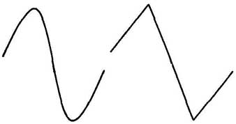
-- (left) Fig. 9 An audio oscillator generates an audio frequency sine wave.
-- (right) Fig. 10 Another common electronic waveform is the triangle wave.
Signal generators
The term signal generator is usually employed for an instrument that produces some waveform other than a sine wave. Typical examples are the triangle wave (-- Fig. 10), the sawtooth wave (-- Fig. 11), and the rectangle wave (-- Fig. 12).
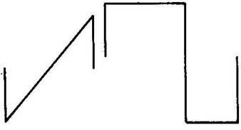
(left) Fig. 11 A sawtooth wave. (right) Fig. 12 A typical rectangle wave.
These different waveforms are useful for different types of tests. A triangle wave is often used in place of a true audio oscillator (sine wave generator) because the required circuitry tends to be simpler and less expensive. Also, the harmonic content of a tri angle wave is relatively weak.
All ac waveforms except the sine wave consist of multiple frequency components. The base frequency is the fundamental frequency, the frequency of the waveform as a whole. It’s the strongest (highest amplitude) frequency component. In simple waveforms, like the ones we are concerned with, the fundamental is also the lowest frequency component.
The other frequency components are called overtones, or harmonics. A harmonic is an exact integer multiple of the fundamental frequency. (Some complex waveforms have enharmonic overtones, which are higher than the fundamental frequency but are not exact integer multiples.) The harmonics are numbered by their integer multiples. For example, if the fundamental frequency is 250 Hz, then the following harmonics are possible:
Harmonics | Hertz
2nd 500
3rd 750
4th 1000
5th 1250
6th 1500
7th 1750
8th 2000
9th 2250
10th 2500
… and so forth, continuing indefinitely.
The harmonics are weaker (lower amplitude) than the fundamental frequency. The higher the harmonic, the weaker its amplitude. The highest harmonics are generally so weak that their effect on the overall waveform is negligible and they can reasonably be ignored. The specific harmonics included and their relative amplitudes determine the waveform.
For example, a triangle wave includes the fundamental and all odd harmonics, but no even harmonics. A square wave includes the same harmonics as a triangle wave of the same frequency, but the amplitude of each individual harmonic is much stronger in the square wave. A sawtooth wave includes all of the available harmonics, both odd and even.
A signal generator that produces rectangle waves is often called a pulse generator. (The terms rectangle wave and pulse wave are generally synonymous.) A rectangle wave has just two voltage levels, HIGH and LOW, with no transition time between the two. (Most other waveforms slide linearly through a range of volt ages.)
Most modern pulse generators feature a control to adjust the duty cycle of the rectangle wave. The duty cycle determines how much of each complete cycle will be in the HIGH state, thus affecting the harmonic content of the waveform. The duty cycle is usually expressed as a ratio, 1 :X. Every harmonic that is a multiple of X’s omitted from the waveform. For example, if the duty cycle is 1:3, every third harmonic will be omitted: Fundamental, 2nd harmonic, 4th harmonic, 5th harmonic, 7th harmonic, 8th harmonic, 10th harmonic, and so forth. Similarly, if the duty cycle is 1:4, any harmonic that is a whole number multiple of 4 will be left out of the sequence: Fundamental, 2nd harmonic, 3rd harmonic, 5th harmonic, 6th harmonic, 7th harmonic, 9th harmonic, and so forth.
The popular and widely used square wave is just a special form of the rectangle wave, in which the level is HIGH for exactly half of each complete cycle. The duty cycle is 1:2; therefore, all harmonics that are multiples of two (all even harmonics) are omitted.
Sometimes you will see a reference to a test instrument known as a signal injector. This is just a simple AF signal genera tor that feeds its output through a probe that can be conveniently moved through the circuit under test to check out various points. Usually a signal generator will have very few controls and features.
Function generators The third major type of AF signal generator is the function generator. A function generator is basically a special form of the signal generator. Most signal generators put out just a single waveshape. A function generator, on the other hand, lets the technician choose from three or four different waveshapes. For certain tests, a square wave , for example, might be better than a sine wave, or vice versa.
Function generators also tend to have a wider frequency range than simple signal generators. Many function generators are capable of putting out signals ranging from a fraction of a hertz up to several megahertz.
RF signal generators
For radio frequency work, an RF signal generator is used. It’s similar in concept to regular (audio and ultra-audio) signal generators, but the output frequency is much higher. The output from an RF signal generator is almost always a sine wave. Usually there is the capability to modulate the main output signal with another signal in the audio range, and the technician can select between amplitude modulation (AM) or frequency modulation (FM).
Because of the high frequencies being produced, an RF signal generator must be very well shielded. Usually it must be type- approved by the FCC. RF signal generators are usually crystal- controlled for accuracy and stability.
==Signal tracers==
A signal tracer is a device for detecting the presence of a signal. Usually it’s not much more than a small amplifier and speaker with test leads for taking its input from the circuit point under test. A signal tracer is often used with a signal generator to test audio equipment, but it can be used alone, also.
A signal tracer is often used in the reverse manner for signal generators. The signal tracer is first connected to the circuit’s out put (usually the speaker terminals). It’s progressively moved backward through the circuit, stage by stage, until the signal has been found. If there is no signal at the output of stage 4, but the signal is fine at the output of stage 3, then the problem is in stage 4.
==Capacitance meters==
Until fairly recently, capacitor testers were not found on too many electronics servicing workbenches for several reasons. The early capacitor testers were bulky and expensive. More importantly, they really weren’t good for very much. Most were basically “go/no-go” type testers that checked for shorts or opens and perhaps gave a rough measurement of leakage. Some of the top units also gave a (very) approximate reading of the capacitance range.
Shorted and open capacitors almost always can be pin pointed in-circuit without a capacitor tester. It also isn’t very difficult to isolate a leaky capacitor with in-circuit voltage and cur rent tests. The early capacitor testers could be handy in certain circumstances, but for most technicians they were an unnecessary luxury. It was nice to have one, but it was no hardship to live without it.
The modern capacitance meter, however, is completely different. It’s essentially a digital device that displays the actual capacitance numerically and with great precision. Most capacitance meters work by measuring the time constant of the capacitor being tested. The time constant is the time required for the capacitor to charge up to two-thirds of the applied voltage through a given resistance. The resistance, of course, is deter mined by the meter’s circuitry and is a constant.
For many applications, the exact value of capacitance is not terribly important. Circuit resistances are usually much more crucial. Most resistors used in circuits today have a tolerance of 5 percent, while 20 percent tolerances are typical for capacitors. However, sometimes a capacitor can change its value outside its tolerance range and throw off circuit performance.
The capacitance value does become crucial in frequency- determining circuits, such as filters, tuners, and oscillators. In some applications, the actual capacitances don’t matter as much as whether or not two or more capacitances in the circuit are closely matched.
A capacitance meter is also useful for hunting down stray capacitances in a circuit. Remember, a capacitor is really nothing more than two conductors separated by a dielectric (insulator). Stray capacitances can show up almost anywhere. Even air can serve as a dielectric. Sometimes stray capacitances are at fault in older equipment that has worked fine for years but suddenly starts behavior erratically. When the stray capacitance is located, it can usually be eliminated by repositioning connecting wires or replacing or adding shielding between the two conductors that are acting like capacitor plates. Adjacent traces on a pc board are particularly prone to stray capacitances.
Another use for a capacitance meter is to test the quality of a length of cable. Most standard types of cable (coax, twin-lead, rib bon, etc.) have characteristic capacitances per foot (or per meter). Just measure the capacitance across the cable and divide by the length to get the specified capacitance-per-unit-length value, or something very close to it.
Capacitance-per-unit-length = Total Capacitance/Length (in number of units
Make sure that you use the same length unit for both halves of the equation.
This equation can also be reversed to get an estimate of an unknown length of presumably good cable.
Length (in number of units) = Total Capacitance / Cap.-per-unit-length
As notice, the modern capacitance meter is a truly versatile and useful piece of test equipment, made possible by digital technology.
==Frequency counters==
It seems the frequency counter is the status symbol for electronics technicians. Everybody wants one, even if they’re not entirely sure what they want if for. If you work primarily in general TV servicing, you probably wouldn’t use a frequency counter very often. On the rare occasions when you need to measure a frequency, you can use your oscilloscope. Just count the number of cycles displayed and divide by the time base.
On the other hand, in some applications a frequency counter can be extremely valuable. Two such applications include musical instrument servicing and working with RF transmitters. In RF transmitters, precise frequencies are required by law. A frequency counter is a handy tool for making sure that oscillators, multipliers, and frequency synthesizers are working properly and are tuned correctly.
All modern frequency counters are digital devices. The measured frequency is displayed directly in numerical form. The typical input impedance of a frequency counter is about I megohm (Me), so loading is minimal. Most commercially available frequency counters measure frequencies up to about 50 MHz or 100 MHz, which should be sufficient for most servicing work. However, if you need to measure higher frequencies, accessory pre-scalers are available to extend the range of a frequency counter.
Servicing test equipment
Any piece of electronic equipment is likely to require servicing sooner or later. Though most people don’t think about it, that obviously includes test equipment.
Conceptually, at least, servicing a piece of test equipment is no more difficult than any other type of electronic circuit. Two special types of difficulties are involved. The first is that some times you need the instrument being tested to perform the necessary tests. Whenever possible, it’s a good idea to have spares of general-purpose equipment, such as multimeters. You need a second multimeter to find a defective component in your first multi- meter. In addition, if you have only one multimeter and it breaks, virtually all of your service work will come to a standstill until you get it fixed.
Multimeters are inexpensive enough that most technicians can afford two or three. The spare units need not be deluxe models with all of the special features of your primary meter. They just need to be sufficient to get you by in an emergency.
Some types of equipment are too expensive to have spares on hand. For example, unless you work in a large shop with several staff technicians, you probably will have just one oscilloscope. If it develops a fault, you will need to borrow or rent one until yours can be repaired or replaced. It’s a good idea to check out the avail ability of an emergency replacement before you are faced with an actual emergency.
VOMs are probably the easiest piece of test equipment to re pair because there really isn’t very much inside them. They are basically made up of switches, a handful of precision resistors, a diode or two, and indicators. Common faults include broken wires leading from the switches, shorts, or burned-out diodes or resistors. Burned-out components are almost always caused by accidentally feeding too high a voltage or current to the VOM or trying to operate it on the wrong range. Trying to measure a moderate to large ac voltage while the meter is set for ohms , for example, almost surely will result in disaster. Unfortunately, this is very easy to do. Almost every experienced technician I’ve ever met has blown out at least one meter at some point in his career.
Unless the over-voltage or current is extremely high, this type of problem is usually fairly easy to repair. It’s just a matter of locating the burned-out component(s) and replacing them. Since there aren’t that many components in the entire VOM circuit, you could test every component individually in just an hour or so. You can make better use of your time, however, by using a little logic to eliminate some of the components as suspects.
In most cases, the damaged VOM will work on some ranges or functions but not on others. Obviously any component included in a working range must be good, so there is no point checking it. Often one or two resistors or diodes will be visibly burned. Some times a burned component looks okay, but can be located by smell, especially right after it was damaged. But don’t rely on eye ball or nose tests alone. Multiple components might have been damaged. A resistor might change value or be internally cracked without being visibly burned. Bad diodes usually can’t be detected without a resistance test of the pn junction. A component that looks bad probably is, but a component that looks good might not be. Don’t be too quick to jump to conclusions.
There is one part of the VOM that is tough to repair: the meter itself. It can be damaged by too large a signal or by a physical shock (such as being dropped). Occasionally, the only problem is a bent pointer needle. If you have a very sure hand, you might try re pairing it. Open up the meter’s housing and carefully bend the meter back into the correct position. Don’t use too much force, or you could break off the pointer needle or bend it irreparably. The pointer needle must be absolutely straight, or the meter will be useless.
In some damaged meters, the driving coil might be burned out. It’s usually not repairable, and the meter itself must be re placed. For a VOM, this usually means buying a whole new instrument, since the meter makes up the bulk of the unit’s cost. Don’t try substituting a cheaper meter unless you are really desperate. An unauthorized replacement probably won’t fit mechanically very well, so it will be more prone to physical damage, and probably won’t last very long. More importantly, its electrical characteristics probably won’t be exactly the same as the original, adversely affect the accuracy of the unit.
VTVMs or other electronic multimeters (FETVMs, etc.) aren’t much more complicated to service, but the circuitry does include one or more active amplification stages. These circuits can be repaired with standard voltage/current measurements and signal-tracing techniques. For some electronic multimeters, it might be worthwhile to order a replacement meter movement from the manufacturer, rather than junking the instrument and buying a new one. Use an exact replacement, or you’ll just be asking for trouble.
Repairing a multimeter isn’t particularly difficult in most cases. In order to put it back into service, however, you must first confirm its accuracy. The unit should be recalibrated after any repair or adjustment. It’s a good idea to perform calibration procedures any time the instrument’s case has been opened. Occasionally, the only repair needed on an apparently defective multimeter is recalibration.
First make sure the meter’s pointer swings smoothly over its entire range. To check this, set the multimeter to one of its ohms ranges. With the test leads held apart, the pointer should be all the way over to the right end of the scale (infinity). Now touch the two lead probes together to create a short. The pointer should swing smoothly to the far left (zero). Bring the leads together and apart several times while watching the pointer closely. It should swing back and forth smoothly without sticking anywhere along its path. If it does stick, the most likely cause is some debris in the pivot base. Open the meter’s housing and carefully remove any foreign matter. You’ll need a sharp eye; any very tiny particle could cause a problem.
Now set the multimeter to a voltage setting and make certain it’s reading the correct value. You need some sort of reference voltage — a battery will do, if it’s fresh. A mercury cell is the best because it holds a very stable voltage, but an ordinary flashlight cell will do if it has never been used or hasn’t been sitting on the shelf too long. A new flashlight battery puts out a reasonably precise 1.56 volts. Adjust the meter’s calibration control (usually an internal trim pot) until the meter displays the correct reading.
An oscilloscope is best calibrated with a square-wave signal of a known level fed to the vertical amplifier inputs. Watch the display closely for any distortion, especially rounded corners. This could be caused by faulty coupling capacitors in the signal path.
Signal generators can be tested with an oscilloscope and/or a frequency counter. Make sure the output frequency correctly corresponds to the nominal frequency of the unit or the setting of the front panel control(s) on a variable unit. On an oscilloscope that is known to be correctly calibrated, check the output wave form for purity, low distortion, and symmetry.
Also see: Component tests