AMAZON multi-meters discounts AMAZON oscilloscope discounts
A small group of extremely useful null circuits are not bridges at all in the conventional sense. They utilize polarities and amplitudes in a-c circuits in such a way that their sum becomes zero (i.e., the circuits null ) at one discrete value of circuit component values and/ or frequency and voltage. Thus, in some applications they provide the same end result that bridges do.
Non-bridge null circuits offer many of the advantages peculiar to bridges-namely, accuracy of measurement, direct reference to a standard, and high resolution. Occasionally they are simpler than bridges. Sometimes they offer additional advantages, such as a common ground between input and output.
This Section describes the principal members of the non-bridge group.
9.1 DC POTENTIOMETER
The d-c potentiometer is a device for the accurate measurement of voltage by balancing an unknown d-c voltage against the precise voltage supplied by a standard cell. Since the cell voltage is on the order of 1.018 volt, most unknown voltages must be stepped down to his value by means of a voltage divider in order to obtain a balance.
Fig. 9-1 shows the basic circuit of a potentiometer. The basis o this arrangement is the voltage divider (potentiometer ) consisting of a length of resistance wire, AB, provided with a sliding contact which moves over a calibrated scale. (Like the scale of the slide-wire bridges described in Sections 2, 3, and 4, this scale may be graduated in inches, centimeters, ohms, or arbitrary linear units.) In some potentiometers, the slide wire is simply a straight length of wire stretched tautly between points A and B, as shown in Fig. 9-1, and situated over or alongside a scale ; in more compact instruments, however, the wire is wound in a ring or spiral around a rotatable drum of insulating material. Meter M is a sensitive center-zero d-c galvanometer. The standard cell is represented by voltage E1> and an external battery by voltage E5 . These two voltages are of the same polarity at point A. Resistor R1 limits the galvanometer current to a safe value and can be removed from the circuit as null is approached. Rheostat R5 allows the current from the external battery to be pre-adjusted.
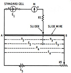
Fig. 9-1. Basic circuit of d-c potentiometer.
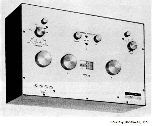
Fig. 9-2. Laboratory-type d-c potentiometer.
Moving the slider along the wire changes the values of R2 and R3 and therefore the ratio of R2 to R4, the full resistance of the slide wire. Corresponding voltages E2 and E3 are proportional to R2 and Ra, respectively. When a voltage E4 is impressed across the slide wire (i .e., between points A and B), the voltage (E2) selected by the slider is proportional to the R2/R4 ratio : E2 = E4 (R2/R4 ) . The potentiometer is balanced first by setting the slider to a trial point along the slide wire, as shown in Fig. 9- 1, and adjusting rheostat R5 for null, as indicated by meter M. At this point, voltage E2 then is equal to the voltage of the standard cell (E1), since the two voltages now cancel each other exactly. This completes the initial adjustment. The standard cell then is removed and the unknown voltage (Ex) connected in its place, the polarity being the same as that of the cell. Unless Ex = E1, the circuit then will become unbalanced, and the slider must be moved to a new point to obtain a second null. This will change resistances R2 and R3, and at this new null setting, the unknown voltage is : where, E1 is the standard cell voltage, R28 is the initial value of R2 at initial balance, R2b is the final value of R2 at rebalance.

9-1
The slide wire may be calibrated to read directly in volts over a somewhat narrow range. Higher voltages may be stepped down through an external, precision voltage divider ( volt box) to fall within the range of the potentiometer. The unknown voltage then becomes :
Ex = e(1/n)
9-2
where, e is the voltage indicated directly by the potentiometer, n is the division factor of the volt box (e.g., if the volt box is set to deliver one-tenth of the unknown voltage, n = 0. 1).
Fig. 9-2 shows a laboratory-type potentiometer (Honeywell Model 2784 ) which offers direct readings of voltage from zero to 11 .1100 volts in four ranges : 0-0.0 111 100, 0-0. 111 100, 0-1 .11100, and Courtesy Honeywell, Inc.
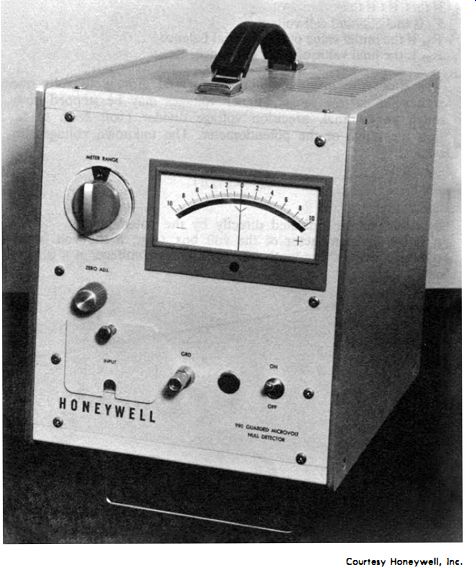
Fig. 9-3. Sensitive d-c null detector used with potentiometer.
0-1 1.1 100.
The slide-wire dial (see center of panel ) has 550 scale divisions for close resolution. Accuracy to ± (0.002% + 10 p,v) is provided. Fig. 9-3 shows the a-c-operated, guarded microvolt null detector (Honeywell Model 3990) which is the companion unit for this potentiometer.
9.2 POTENTIOMETRIC VOLTMETER
The potentiometer principle described in the preceding section may be used in a d-c voltmeter which, using a precision variable resistor and the null method, can furnish higher accuracy than is obtainable with the meter method of measurement. The reason is that, at null, the instrument draws no current from the unknown voltage source, and therefore offers zero loading (infinite resistance ). Fig. 9-4 shows the basic circuit of this type of instrument. Here, the unknown voltage (Ex ) is applied to the potentiometer, and the resultant output voltage (Eo) is proportional to the position of the wiper along the resistance element (i.e., upon the resistance ratio R3/ R1 ). Meter M is a center-zero d-c galvanometer, and Es is a standard voltage derived from a standard cell, mercury battery, or voltage-regulated supply.
The applied and standard voltages are applied to the meter in polarity, so that the deflection is zero when the potentiometer is adjusted to make Eo = Es. At this null point, the unknown voltage may be determined from the resistance ratio and standard voltage : 9-3 In practice, the potentiometer is calibrated to read directly in volts. High resolution is obtained through the use of a series of decade resistors or a precision, multiturn potentiometer. Alternating voltages may be measured if a suitable rectifier is operated ahead of the INPUT terminals, and corrections made for the rectifier performance.
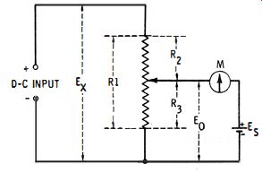
Fig. 9-4. Basic potentiometer voltmeter circuit.
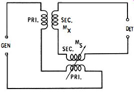
Fig. 9-5 Felici mutual-inductance balance.
9.3 FELICI MUTUAL-INDUCTANCE BALANCE
Fig. 9-5 shows a null circuit (Felici mutual-inductance balance) for checking an unknown mutual inductance (Mx) in terms of a known standard one (Ms). The two double-coil inductor units are so situated that no mutual inductance exists between them, and the secondary windings must be connected in phase opposition. Continuously variable mutual-inductance standards are available. One such device (General Radio Type 107-N) provides a range of 0- 110 mh at ± 2.5% accuracy (related to full scale). The circuit IS balanced by adjustment of standard inductor Ms.
At null :
9-4
Unlike the Carey-Foster circuit (Section 4. 13, . Section 4), the Felici arrangement is not a true bridge.
9.4 BRIDGED-T RC NETWORK
The resistance-capacitance null circuit shown in Fig. 9-6 is termed a bridged T from the bridging effect of resistor R 1 across the T network C1-C2-R2. With a given set of R and C values, the phase relations at one frequency are such that a signal applied to the input (GEN) terminals is canceled at the output (DET) terminals.
This circuit does not give a true null; i.e., the output voltage at balance does not fall completely to zero. But it does reach a low minimum in most cases, especially when R1 is very high with respect to R2. If C1 is kept equal to C2, then at balance : where, f = v'1 I( R1 R2)
27TC
C equals C1 or C2 in farads, f is in Hz, R is in ohms, pi equals 3.1416.
9-5
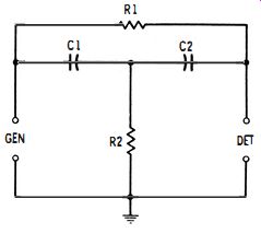
Fig. 9-6. Bridged-T r-c network.
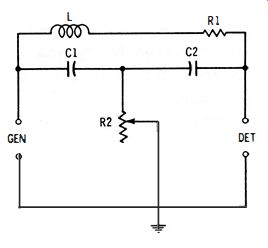
Fig. 9-7. Bridged-T l-c network.
The circuit is used sometimes to check a high resistance (R1) in terms of a known low resistance (R2), especially at high frequencies. In this application, C1 and C2 are varied simultaneously and have the same capacitance at all settings. At balance:
The advantage of the bridged-T circuit is its relative simplicity and its provision of a common ground for the generator, network, and detector. This latter feature removes the need for a shielded transformer at either the input or output and reduces cross coupling and pickup. It also permits operation of the network at radio frequencies.
9.5 BRIDGED-T L-C NETWORK
Another bridged-T circuit is shown in Fig. 9-7. In this one, an inductor (L) bridges the T network (C1-C2-R2 ) in the same manner that a resistor bridges the T in the preceding section. In the inductive leg, R1 is the equivalent series resistance of the inductor and has a low value in the high-Q inductors preferred for this circuit.
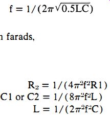
The capacitances C1 and C2 are made equal and may be varied simultaneously to tune the network. (Alternatively, the capacitors may be maintained equal and fixed, and the inductance varied.) To balance the network, the capacitance (or inductance ) and resistance R2 must be adjusted alternately. Unlike the R-C bridged-T network, this L-C version gives a complete null. At balance:
f = 1/ (21TVO.5LC) where, C equals C1 or C2' in farads, f is in Hz, L is in hy, 1T equals 3. 1416.
Rz = 1/ (41T2fZ R1)
C1 or C2 = 1/ ( 81T2f2L )
L = 1/ (21T2FC)
9-7
9-8
9-9
9-10
The bridge-T circuit is used for the measurement of inductance and capacitance at frequencies as high as the lower vhf spectrum, and it is used also as a band-rejection filter (notch filter) . An advantage of the bridge-T network is its provision of a common ground for generator, network, and detector. This removes the need for a shielded transformer at either the input or the output, thus reducing cross coupling and pickup and permitting operation at high frequencies.
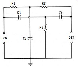
Fig. 9-8. Twin-T (parllllel-T) network.
9.6 TWIN-T (PARALLEL-T) NETWORK
This resistance-capacitance null network (Fig. 9-8 ) takes its name from the fact that it consists of two T's ( R1-R2-C3 and C1-C2-R3 ) connected in parallel. It gives a complete null, and its passband is reasonably narrow if high-Q capacitors are used and if the network is driven from a low impedance and loaded with a very high impedance.
The behavior of the twin-T network is similar to that of the Wien bridge (Section 7.3 ), but its selectivity is significantly better.
The twin-T, in common with other frequency-selective networks, may be balanced at only one frequency at a time, and this frequency is determined by the resistance and capacitance values, as in the Wien bridge. Conversely, at a fixed frequency, resistance and capacitance values may be determined with the aid of the twin T. In the twin T, as in the Wien bridge, there are many combinations of resistance and capacitance which will result in balance at a given frequency. The balance equation is greatly simplified when the network is symmetrical-i .e., when C1 = C2 = lhC3, and R1 = R2 = 2R3 . Under these conditions, at null : where, C1 is in farads, f is in Hz, R 1 is in ohms, 7Tequals 3.1416.
f = 1/ (2 pi R1C1 )
9-11
In the Wien bridge, two capacitances or two resistances must be varied simultaneously to tune the circuit over a range of null frequencies. In the twin-T network, three capacitances (C1l, C2, and C3 ) or three resistances ( R1, R2, and R3 ) must be varied simultaneously. This sometimes makes the continuously variable twin T difficult to actualize, since three-gang rheostats or variable capacitors with a high degree of tracking are hard to make and therefore expensive.
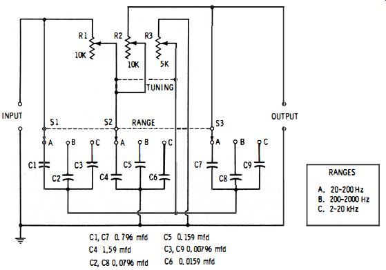
Fig. 9-9. Twin-T a-f meter.
The twin T, like the bridged-T network, provides a common ground for generator, network, and detector, thus removing the need for a shielded transformer at either the input or output and thereby reducing cross coupling and pickup, as well as permitting operation at radio frequencies.
The twin T is widely used as a band-rejection filter (notch filter) and is used occasionally to check capacitance or impedance (shunted across C3 or R3 ) at high frequencies. It is advantageous as a null type frequency meter similar to those described in Section 7.3. Fig. 9-9 shows the circuit of a twin-T audio-frequency meter which covers the range from 20 to 20,000 Hz in three steps : 20-200 Hz, 200-2000 Hz, and 2-20 kHz. Tuning is accomplished with a three-gang wire wound rheostat having two 10000-ohm sections ( R1 and R2 ) and one 5000-ohm section (R3 ). Ranges are changed by the three-pole, three-position switch (S 1-S2-S3 ), which selects closely matched capacitors (C1 to C9 ) in threes. A high-impedance detector must be used (e.g. , oscilloscope, a-c vtvm, ' or magic-eye tube ).
9.7 HALL NETWORK
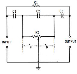
Fig. 9-10. Hall network.
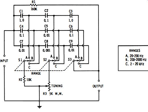
Fig. 9-11. Tunable Hall network.
The Hall network (Fig. 9-10) is a resistance-capacitance circuit in which continuously variable tuning is obtained with a single potentiometer, R2. In this respect, this circuit is superior to the
Wien bridge and twin-T network, both of which require that several components be simultaneously variable and well tracked. Like the bridged-T and twin-T circuits, the Hall network provides a common ground for the generator, network, and detector (load). Also, like the preceding circuits, the Hall network may be balanced for only one frequency at a time.
Three capacitors (C1, C2, and C3 ) must be switched together to change tuning ranges, and the relationship C1 = C3 = lOC2 must be maintained in each range. At null:
… where, C is in farads,
f. is in Hz, r is in ohms, 1T equals 3. 1416.
f= 9-12
The Hall network finds its principal use as a band-rejection filter (notch filter), its response curve being similar to that of the twin-T network. It may also be used, similar to the Wien bridge and parallel T, as an audio-frequency meter. Fig. 9-11 shows a continuously tunable Hall network which covers the range from 20 to 20,000 Hz in three steps : 20-200 Hz, 200-2000 Hz, and 2-20 kHz. The 5000-ohm wirewound rheostat, R3, is the tuning control. The ranges are changed by the three-pole, three-position switch, S1 -S2-S3, which selects the capacitors in threes : C1 -C2-C3, C4-C5-C6, and C7-C8-C9.