AMAZON multi-meters discounts AMAZON oscilloscope discounts
To more fully understand the theory of capacitors, especially how they perform in actual operation, it is necessary to analyze the effects of the different conditions to which they will be subjected.
Fig. 2-1A shows a theoretically perfect capacitor. The equivalent circuit of an actual capacitor, as shown in Fig. 2-1B, indicates there are other characteristics besides capacitance to be considered. There is the inductance L of the leads and plates, resistance R1 of the dielectric (leakage resistance), resistance R2 of the leads and plate material (effective series resistance), and measured capacitance C.
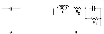
Fig. 2-1. Theoretical and equivalent circuit of a typical capacitor.
ENERGY ABSORPTION
Whenever a capacitor is charged or discharged, work is performed; in other words, energy must be expended. It takes a certain amount of voltage to produce enough current to charge a capacitor, and the product of amperes and volts is watts, which is the unit of power. This power must be expended in some way. Most of it will be held in reserve until the capacitor is discharged. This will represent the major portion in a good-quality capacitor. The remainder of the power, however, will be dissipated in the form of heat. This is caused by the PR loss in the resistance R2 (Fig. 2-1B) of the leads and plates of the unit. PR losses take place during both the charge and discharge cycles.
Obviously, this heat loss must be held to some reasonable level. Therefore, it is often necessary to make a capacitor larger than mere electrical requirements would seem to dictate.
The heat produced during the charge and discharge cycles results from the fact that there is no such thing as a perfect capacitor. If there were, all the energy it receives would be stored there for future use. The more rapidly a capacitor is charged and discharged, the more critical these internal losses become. In fact, heat can build up to the point where the capacitor can be damaged.
POWER FACTOR
Power factor is the term used to describe the ratio of power lost to the total power used to charge a capacitor.
It is a rather complex function involving all the losses en countered, and depends on frequency, temperature, dielectric material, voltage stress, and the resistance of the leads and plate material. Let's take a look at these factors to see how they affect power factor.
Everything in nature has a tendency to vibrate, and the vibrations will occur more freely at one frequency than at any other. Witness the window glass rattling as an airplane passes overhead, or the singer cracking a crystal goblet with a high C note. These are examples of mechanical vibrations to which some capacitors may be subjected under certain circumstances. Such vibrations can result in a change of capacity as the distance between the plates varies at its natural (resonant-frequency) rate.
The greater effect in capacitors, however, is electrical in nature. When an inductor and capacitor are placed in series, they form a resonant circuit which has the property of offering a very low opposition to the flow of a changing (alternating) current at some particular frequency, but maximum opposition at all others. The frequency at the point where this opposition is lowest is known as the resonant frequency of the circuit.
So how does all this affect capacitors? As the resonant frequency is approached, apparent capacitance drops off very sharply and power factor increases rapidly. Here's an example of what we're talking about. Suppose we are re placing a capacitor in a circuit which handles a frequency of 2,000 khz. The original unit was rated at 0.1 mfd, 600 VDC. Can we replace it with one, which just happens to be there on the bench, rated at 0.1 mfd, 3,000 VDC? Not necessarily, because the resonant frequency of the original was selected to be well above 2,000 khz, whereas the resonant frequency of the second could very well be at or near 2,000 khz. Use of this second unit would be wasted effort, because it could quickly overheat and fail.
A second important frequency consideration is lead length. The shorter and thinner the leads, the higher the resonant frequency becomes. Let's take another example, involving 5,500 megacycles. The original unit was rated at 0.01 mfd and its leads were one-half inch long. It is in a particularly awkward spot, so we'd like to install a re placement unit with 2-inch leads for convenience. Can we do it? Again, not necessarily. The half-inch leads have a resonant frequency well above the signal frequency in our circuit, but the 2-inch leads may resonate near 5,500 mhz.
This could result in rapid capacitor deterioration, meaning we'd just have to do the job over.
The conscientious technician will always remember to re place capacitors with the same type, and to install them as nearly as possible like the original unit. This is especially true in highly critical circuits and/or where frequencies are relatively high.
TEMPERATURE
Capacitors are affected more by temperature than by any other environmental condition ( except humidity). Capacitors are rated at a particular temperature, most generally 25°C. Any deviation from this temperature will change their capacitance and voltage rating.
As the temperature increases beyond 25°C, the capacity also increases, but the voltage-breakdown resistance decreases. On the other hand, a decreasing temperature does just the opposite--it decreases the capacitance and increases the voltage-breakdown resistance. In both instances the power factor will increase. In short, most capacitors perform best at approximately 25°C; any deviation will adversely affect their performance.
The preceding paragraph is to be considered only a general rule; there are exceptions, of course. Many capacitors, particularly ceramic types, are specifically designed to de crease in value with an increase in temperature. A description of this type will be found in Section 3.
The principal reason a rising temperature has such an effect on capacitor operation is that electron activity increases also. Thus, at 25°C a dielectric gap could be sufficient to prevent a breakdown at 450 VDC, but at 100°C the capacitor might rupture.
-----------------
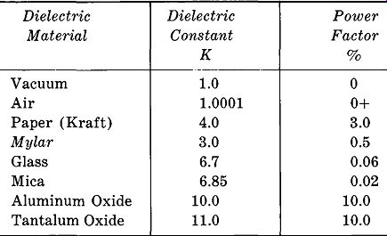
Table 2-1
Dielectric constants and power factors of common dielectric materials.
Dielectric
Dielectric Power Material Constant Factor
K % Vacuum 1.0 0 Air 1.0001 o+ Paper (Kraft) 4.0 3.0
Mylar 3.0 0.5
Glass 6.7 0.06 Mica 6.85 0.02
Aluminum Oxide 10.0 10.0
Tantalum Oxide 11.0 10.0
----------------
DIELECTRIC MATERIAL
Dielectric material characteristic is also affected by a change in temperature. The relative merits of various materials were discussed in Section 1, but only from a di electric or insulating standpoint. Now let's examine these materials from a power-factor standpoint. It must be emphasized that the values in Table 2-1 are only approximate; they may vary in specific cases.
It is interesting to note that although Mylar has only a slightly lower dielectric constant than paper, its power factor is substantially lower. As a result, though its dielectric might have to be slightly thicker, a Mylar capacitor should have lower internal losses than its equivalent paper unit.
The more common dielectrics tend to become less effective as their temperature increases. The lower efficiency adds to the already increased electron activity and in this way hastens voltage breakdown.
You will note that Table 2-1 does not include ceramics.
There is no standard ceramic dielectric; each one is specially formulated to suit a particular application.
DIELECTRIC STRESS
Too high a voltage will weaken the dielectric strength of an insulator. Thus, a dielectric rated at 600 VDC will probably break down at 1,600 VDC. Even though a break down doesn't occur at the higher potential it will leave the dielectric susceptible to future failure at even its rated voltage.
As would be expected, an important factor involved in dielectric stress is the quality of the dielectric itself. Im purities, especially if they are metallic, can produce areas of poor resistance and result in breakdown. During the manufacture of paper capacitors, minute amounts of impurities will creep into the fibers of the paper pulp, even with the most careful quality control. To minimize the alignment of these conductive particles, paper capacitors are commonly constructed of layers upon layers of paper.
Dielectric stress is expressed in terms of volts per mil (.001 inch) thickness-the better the dielectric, the higher the volts per mil. However, this figure will decrease as the temperature, frequency, and/or thickness of the material increases.
PLATE LOSSES
The over-all performance of a capacitor depends on a wide variety of factors. Of these, dielectric efficiency is of primary importance, but the efficiency of the plates (conductors) cannot be overlooked. The choice of plate material must of necessity be a compromise. Copper would be the obvious choice electrically, but it corrodes easily and is relatively less stable than aluminum. Aluminum, therefore, has become the most common plate material in spite of slightly less conducting ability. Silver and tantalum are used where their advantages outweigh their added costs.
The efficiency of plate materials decreases as temperature increases because of added conductive resistance. In addition, the efficiency of the dielectric decreases. Many other factors are involved, but generally, over-all losses increase as temperature increases and vice versa. In spite of this, many capacitors exhibit increased capacitance as temperature increases. But, the over-all losses are higher and over-all efficiency is lower.
EQUIVALENT CAPACITOR CIRCUIT
Let's return to the equivalent circuit of a capacitor. While the perfect capacitor would have no losses of any sort, and would merely represent an energy potential inserted in any given circuit, an actual unit unfortunately has several imperfect characteristics.
Every conductor possesses a certain amount of inductance. A conducting wire or the flat plates of a capacitor will exhibit minimum inductance. By rolling the plates into a cylinder, the inductive value will increase. A further increase will result by rolling the plates into a coil-more turns produce a higher inductance.
A perfect capacitor would have an infinite resistance.
In actual practice, however, all capacitors have a certain amount of leakage, which an ohmmeter will show as a resistance. The amount of this leakage resistance (R1) will vary from one type and value of capacitor to another. It may range from 1,000 megohms in one unit, down to 50K in another. Yet both units may be performing satisfactorily.
This matter of capacitor leakage is covered more fully in Section 6.
The effective series resistance (R2) of a capacitor is actually a combination of the lead and plate losses and is generally much lower than the leakage resistance. It is useful only in calculating the over-all efficiency of a capacitor.
CAPACITANCE MEASUREMENT
By definition, a capacitor is a device capable of temporarily storing electrical energy. That is, the device is said to have capacitance.
How does one measure capacitance? One way is to compare the capacitor against a known standard by means of a bridge circuit. Another is to use a wattmeter, which measures the actual amount of energy. The latter is probably the only true means of fulfilling the requirements of the following formula for capacitance: where, C is the capacitance in farads, Q is the quantity of charge in coulombs ( one coulomb is equal to a current of one ampere flowing for one second), V is the voltage across the capacitor plates.
As an example, assume we charge a capacitor to 500 volts and then discharge it through a sensitive watt/second meter, getting a reading equivalent to one ampere/second of current flow. Solving the equation, we find that C = 1/500, or .002 farad (2,000 mfd).
The time-constant method is another way of measuring capacitance with substantially the same accuracy. A circuit diagram of this method is shown in Fig. 2-2.
(Q)sroewmH DC VTVM -=- E R
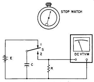
Fig. 2-2. Circuit for use in the time-constant method of capacity measurement.
This admittedly is a rather crude test, since a stopwatch is used, but it serves to depict the principle involved. E is the energy source, S is a single-pole-double-throw switch, R is a 1,000-ohm resistor, and C is the capacitor under test.
A sensitive vacuum-tube voltmeter, with an input resistance of a least 1,000 times the value of R, is used for the voltage readings.
While the switch is in position 1, the capacitor remains charged. To start the test, we simultaneously depress the switch to position 2 and start the stopwatch. When the VTVM reads approximately 37% of the maximum voltage reading, we stop the watch. Capacitance can now be calculated from the following equation:
t C=R
... where, C is the capacitance in farads, t is the time in seconds, R is the resistance in ohms.
For purposes of illustration, assume two seconds has elapsed. The equation is solved to give C = 2/1000, or .002 farad (2,000 mfd). If the time had been one second, the answer would have been 1,000 mfd, and so on.
This test is only as accurate as the timing method used.
The one described would be useless for small capacitors.
However, by substituting an oscilloscope equipped with a millisecond timing pulse, we could achieve a high degree of accuracy.
CAPACITOR OPERATION
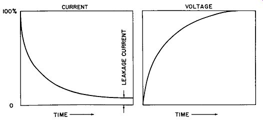
Fig. 2-3. Capacitor charging characteristics.
A capacitor does not charge or discharge at a steady rate.
At the first instant that voltage is applied, the capacitor will have the least amount of opposition to electron flow. There fore maximum current will start flowing. As electrons accumulate on one plate of the capacitor, it becomes more and more difficult to add others. Finally, the point is reached where the available force (voltage) will no longer be able to increase the charge, and the capacitor will be fully charged. To put it in another way, let's go back to the first instant, just as current starts to flow. No voltage difference exists across the capacitor (no excess electrons), but as electrons rush to one plate and withdraw from the other, they produce a potential which opposes the applied voltage. There is less voltage difference existing now, so a reduction in current flow takes place. In other words, the more the capacitor charges, the greater the opposing voltage becomes-until finally it reaches the same value as the applied voltage and current flow ceases. The action occurs at an exponential (nonlinear) rate. Fig. 2-3 illustrates the typical response of a capacitor to a charge cycle.
Notice that the current flow reaches maximum almost instantly, but diminishes gradually to minimum. It never reaches absolute zero, which is an indication of the leakage current; if the capacitor were perfect, the current would drop to zero. The voltage rises in a manner similar to the current decrease, except it finally reaches a maximum value and remains there as long as voltage is applied to the capacitor.
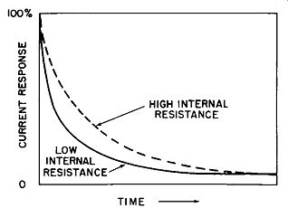
Fig. 2-4. Comparison of charging current response.
The speed with which a capacitor charges is a function of its size ( or capacity) and the external and internal resistances. If we have two capacitors of equal value, but one has a low and the other a high internal resistance, the comparison would be similar to Fig. 2-4.
You will note that the current finally decreases to the same level in the higher-resistance capacitor, but takes longer to do so. The actual lag between the two may be only a small fraction of a second, but even this difference can be critical in a high-frequency application. The reason is that the capacitor must be able to respond to the frequency of the applied voltage at a given rate. If the time response of the capacitor changes, the entire circuit operation could be upset.
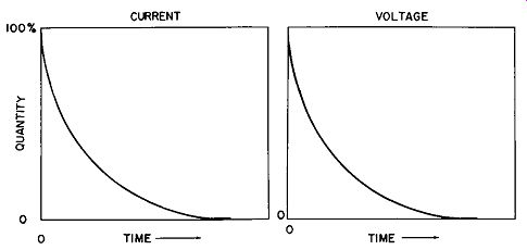
Fig. 2-5. Capacitor discharge response.
When a capacitor is discharged, the response curve is as shown in Fig. 2-5. Now the current and voltage responses are the same. The discharge of a capacitor is very rapid at first, and then tapers off until the device is apparently completely void of charge.
Perhaps you have experienced this situation--a capacitor, which you are certain has been completely discharged, suddenly shows a charge again--and have wondered why.
Let's take another look at the discharge characteristic of a capacitor, but this time we'll expand the time scale as shown in Fig. 2-6.
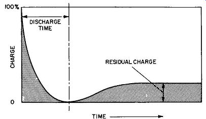
Fig. 2-6. Discharge curve with residual charge shown.
Here we have discharged the capacitor briefly, until it apparently has no charge left. Then we place it to one side.
Gradually the charge seems to rebuild until it reaches a definite level. If we now check, we will verify that a small charge has been retained by the capacitor. The reason is that not all of the electrons were evenly redistributed during the discharge operation. This phenomenon is referred to by engineers as dielectric absorption. All materials have atomic structures, and all atoms have electrons in orbit around a nucleus. The freedom with which one or more of these electrons enter or leave their orbits determines the relative merit of a material as a conductor.
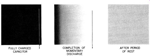
Fig. 2-7. Illustration of capacitor residual charge.
Application of voltage across the dielectric causes the electrons to be redistributed so that more of them accumulate near the positive plate and less near the negative plate.
This stressing of the dielectric occurs upon initial application of voltage and, in effect, "forms" the dielectric. Never again will the material be the same as it was before the potential was applied. When the capacitor is allowed to discharge, most of the electrons will try to redistribute themselves evenly. But those in the dielectric are "held" fairly tightly, a condition that predominates in insulators.
Fig. 2-7 shows the principle involved. A fully charged capacitor is shown as having a dense accumulation. At the time of discharge most of them move from the capacitor as shown by the arrow. Some, however, are firmly entrenched, and will not leave their orbits of their own volition. Thus, it is impossible to ever completely discharge a capacitor once it has been subjected to a DC charge.
TIME CONSTANT
Mention has been made, throughout this section, of the charge and discharge cycles of a capacitor. In each instance time has been a factor. This was taken into consideration in the problem of capacitance measurement, but further examination will be helpful.
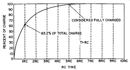
Fig. 2-8. Charge on capacitor at various RC times.
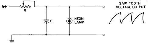
Fig. 2-9. Circuit of neon sawtooth generator.
The formula C = t ...,... R, used in solving for the capacitance value, is also the one we will use to explain RC time constants. Expressed in terms of time, the formula becomes t = RC; t being time in seconds, R resistance in ohms, and C capacity in farads. The definition of the term time constant (1 RC time) is the length of time required to charge a capacitor to 63.2% of the applied voltage. It is further recognized that at the end of 5 RC times, the capacitor will be considered fully charged. Fig. 2-8 shows this graphically.
Since resistance is always present-whether deliberately introduced or contained in the internal structure of the capacitor-the RC time constant must always be considered.
The discharge is governed by the same rules as the charging rate. Often the circuit is designed to have a different resistance on the charge than on the discharge cycle. This means the time constants will be different. An example of this is illustrated in Fig. 2-9. The capacitor is charged through a relatively long time-constant and discharged through a very short one. When the voltage is first applied to this circuit, the potential across the capacitor starts rising from zero, at a rate determined by the values of R and C. If allowed to continue, it would reach the applied voltage in approximately 5 RC times. Before it reaches this point, however, the firing or ionizing potential of the neon lamp is reached and the capacitor now starts discharging through the very low resistance of the ionized neon, meaning the rate will be much more rapid. At some point, deter mined by the characteristic of the lamp, the voltage will have decreased to the de-ionizing potential of the neon, the lamp becomes an open circuit, and the capacitor again starts charging through resistance R, toward the applied voltage.
This action is repeated as long as the voltage is present, producing the series of sawtooth waveforms shown in Fig. 2-10.
The repetition rate, or frequency, of this sawtooth is governed by the values of R and C and by the characteristics of the neon lamp. In the circuit shown in Fig. 2-9 the value of resistance R is varied to change the frequency.
CAPACITIVE REACTANCE
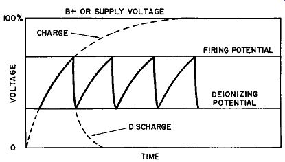
Fig. 2-10. Voltage variation on capacitor in neon sawtooth generator.
In the charging of a capacitor, opposition to the flow of electrons is present in the form of resistance and the natural reluctance of the dielectric to accept them. As long as only DC voltages are involved in the charging process, the latter factor is a constant for a given unit. In applying alternating voltages, however, this second factor becomes variable, its value determined by the frequency of the alternations. It is known as capacitive reactance, and opposes the flow of electrons in the charge-discharge process. Like resistance, it is measured in ohms. In applying an AC voltage, a capacitor is first subjected to an attempt at being charged in one direction and then, a short time later, in the opposite direction. This means the capacitor is charged toward a positive potential, discharged back to zero, charged toward an equal negative potential, and again discharged back to zero--this action repeating itself as long as voltage is applied.
The length of time the capacitor has to attempt the charge or discharge is determined by the frequency of the applied voltage.
Capacitive reactance is expressed by the formula:
1 Xe= 2 pi fC
… where, X,. is the capacitive reactance in ohms, f is the frequency in cycles per second, C is the capacity in farads.
From this formula it can be seen that the higher the frequency and/or capacity, the lower the reactance becomes.
As the frequency is decreased the reactance increases, until the condition corresponding to zero variation in the applied voltage--in other words, DC--is reached. Here the reactance has reached infinity, as evidenced by the fact that no electrons are flowing because the capacitor has had time to become fully charged.
When frequencies are high with respect to the time constant of a particular R-C circuit, a condition will exist where the capacitor will neither charge nor discharge appreciably.
In other words, the time for the voltage to change from zero to maximum permits the capacitor to accept only very few electrons. Therefore, very little of the alternating voltage potential will ever exist across the capacitor. Instead it will appear across the associated resistance. This would be an example of a good coupling circuit, such as shown in Fig. 4-5, where nearly all the alternating (signal) voltage will appear across R,0 to be amplified by V2.
IMPEDANCE
In circuits consisting of resistance and capacitance, another term is used to denote the total opposition to electron flow when an AC voltage is present. This is called impedance, represented by the symbol Z, and is a combination of resistance R (which remains constant regardless of frequency) and the capacitive reactance (which does not). When the resistance and capacity are in series, impedance is computed from the formula
Z = yR2 + X/, where Z, R, and Xe are in ohms.
An example utilizing both the impedance and capacitive reactance formulas will point out the variation existing at two different frequencies. Let us find the impedance of a 100-ohm resistor in series with a 0.1-mfd capacitor at 1,000 hz, and then at 10,000 hz. First we must find the capacitive reactance:
At 1,000 hz: 1 X,. = 2 pi fC X = 1 " 2 X 3.14 X 1,000 X .0000001 = 1,590 ohms
At 10,000 hz: X = 1 ,. 2 X 3.14 X 10,000 X .0000001 = 159 ohms
Notice that X" is 10 times greater at 1,000 than at 10,000 hz, illustrating that capacitive reactance is inversely proportional to frequency. Now using our impedance formula:
At 1,000 hz:
At 10,000 hz:
Z = ?100~ + 1590~
= y2,540,000
= 1,593 ohms
Z = ylOO~ + 159~
= 35,300
= 188 ohms
Notice here that the impedance change is not proportional.
This condition can be directly attributed to the addition of the resistive element.
These results show that a different opposition to electron flow exists for each frequency involved.
RESONANCE
Capacitors in combination with inductors form circuits capable of discriminating between different frequencies.
These are generally known as tuned, or resonant circuits because they respond only to frequencies in the resonant range. Where a range of selection or rejection is desired, variable capacitors or inductors are employed.