BY ERNO BORBELY, Contributing Editor
We MAKE MEASUREMENTS on audio equipment for any number of reasons. The designer must know if his design is going to meet the final product ’s design goals. The manufacturing engineer must ensure that all products coming off the line will meet the specifications. The service engineer must diagnose problems and, after repairs, check that the unit still meets the original specs. Finally, the end user--you or a reviewer--might want to check the claims of the manufacturer.
The difficult part of any audio measurement is correlating it with the sensations of the human ear. Just to mention one measurement with which we are all familiar, total harmonic distortion (THD) is commonly used to evaluate the ‘sound quality’ of a sound system. However, it has been demonstrated that a sound system with a low value of THD can be perceived as having higher distortion than the one which actually measures a higher THD! In spite of an inconsistent relation between THD measurements and auditory sensation, the measurement is useful, as we will see later.
Why Audio Measurements?
Let ’s now-briefly-look at the reasons to measure an audio system in the first place. A block of audio equipment (Fig. 1) is driven by an input signal, which, strictly speaking, is a music signal, but for the sake of this discussion can be a sine wave, a square wave, Or any combination of signals. The output signal, amplified, converted to some other type of signal through transducers and so on, should ideally be an exact replica of the input signal. If it is different in any way from the input signal (besides the amplification; conversion and so forth), it is said to be distorted.
------------------
ABOUT THE AUTHOR
Erno Borbely is currently employed by National Semiconductor as its training manager for Europe. He received a degree in electronic engineering from the Technical University of Norway in 1961 and worked for the Norwegian Broadcasting Corporation designing professional audio equipment for seven years. He lived in the US and was director of engineering for Dynaco and The David Hafler Company. From 1973-78 he worked for Motorola Geneva, Switzerland, as senior applications engineer.
-----------------
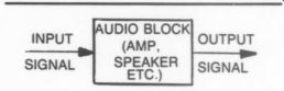
FIG. 1: AUDIO BLOCK SPEAKER ETC.) SIGNAL.
In the widest sense this might include a kink in the frequency response, a time delay between the different frequency components or an extra harmonic or two added to the original signal. When we try to be more specific, it turns out that all distortions can be grouped into two categories: linear and nonlinear.
Linear distortion occurs when the relative relationships of the signal ’s components are changed either in amplitude (intensity), or phase (timing), compared to the different frequency components of the original signal. ’ Quantitatively, the relative changes are presented in the form of graphs, showing amplitude (or gain) vs. frequency, and/or phase vs. frequency. Although we are sensitive to changes in amplitude and phase, linear distortions can, in principle, be corrected (equalized) by appropriate filters.
Nonlinear distortion changes the harmonic content of the original signal through its (nonlinear) transfer characteristics. Figure 2 shows the transfer characteristics of an ideal device; it is a straight line, where the slope indicates the gain of the device. For a device with such a characteristic, the output can be described with the following equation:
V_out = A1 (Vin) (1)
where A1 is the slope (or gain) of the device. Unfortunately, such an ideal device doesn’t exist. All physically realizable audio devices (microphones, amplifiers, speakers) have a nonlinear transfer characteristic, which will introduce second-order, third-order and so forth, components into the original signal. Nonlinear distortion can, at least theoretically, also be removed from the signal, but this is difficult to accomplish.
A device with nonlinear transfer characteristic can be described with the following power series®*:
V_out = A1(Vin) + A2(Vin)^2 + A3(Vin)^3 + A4(Vin)^4 + A5(Vin)^5 +... (2)
The terms A2, A4, and so forth, are even-order nonlinearities; A3, A5, and
so on, are odd-order nonlinearities. A2, A3, or whatever, can be real, constant
and frequency independent, causing what we call static distortion. however,
they can also be complex, amplitude and frequency dependent coefficients,
and this results in dynamic distortion. 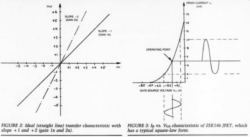
FIGURE 2: Ideal (straight line) transfer characteristic with slope +1 and
+2 (gain 1x and 2x).
FIGURE 3: Ip vs. Vgs characteristic of 2SK146 JFET, which has a typical square-law form.
Static Distortion
Although present in practical devices, the terms beyond the third-order are of diminishing importance, and equation (2) can be truncated to:
Vout = A1(Vin) + A2(Vin)> + A3(Vin) (3)
Furthermore, some devices exhibit dominantly second-order or square-law characteristics (the A2 term is dominating), whereas others have predominantly third-order or cubic characteristics (the A3 term dominating). Let ’s look at a square-law characteristic of the form for a moment:
Vout = A1(Vin) + A2(Vin)? (4)
Assuming that we apply a sine wave (for mathematical purposes we actually use a cosine) to the input:
Vin = V cos wt (5) then Vout becomes:
V_out = [(A2 x V?)/2] + A1 x V cos wt + [(A2 x v^2)/2] cos et (6)
As you can see, the input signal has been significantly altered at the output as a result of the second-order nonlinearity. The first term is frequency in dependent, representing a DC term, the second term is the amplified input signal and the third term is a second harmonic of the input signal.
With two sine waves of the form: Vin = V1 cos wlt + V2 cos w2t, the output will, in addition to two DC terms and two second harmonic components, also contain two intermodulation (sum and difference) products:
A2 x V1 x V2 cos(w1 -w2)t + A2 x V1 x V2 cos(wl +w2)t (7)
A typical square-law characteristic plotted in Fig. 3 shows the transfer characteristic; Ip vs. Vgs, of a 2SK146 JFET. If you want to operate a single FET in a linear amplifier configuration, you must bias the FET in the ‘linear region’ of the characteristics (see operating point). If you apply a sinewave to this amp’s input it will cause a variation in the drain current which is severely distorted; the bottom side of the curve is flat compared to the upper side. The square-law characteristic produces a second harmonic component in the signal.
To avoid second-order distortion, de signers invented differential amplifiers, push-pull amplifiers and bridge-amplifiers. This technique pushes A2 toward zero, by making the transfer characteristics symmetrical around the operating point.
A typical example of such a symmetrical transfer characteristic is shown in Fig. 4, taken from my description of the differential amplifier (TAA 5/83, p. 8).
This type of characteristic has a cubic term with A3#0. Cubic nonlinearity will produce a third harmonic with single sine wave input and so-called third-order intermodulation products with two sine wave inputs. These intermodulation products have frequencies of: 2f1 -f2, 2f2 -f1, 2f1 +f2, and 2f2+f1. With f1 = 9kHz and f2 = 20kHz, intermodulation products will be produced at 2kHz, 31kHz, 38kHz and 49kHz. Of these, the 2kHz product is the important one because it is in the middle of the audio band. Other frequency combinations might produce more than one or, worst case, all beat frequencies in the audio band.
If you apply more than two sine waves to a device with cubic nonlinearity you will end up having an increasing number of intermodulation products. For example three sine waves will produce triple beat products of the type: f3-f2 - f1, which is often used in inter modulation measurements.
As we discussed earlier, the coefficients A2, A3, and so on, can be real, constant and frequency independent.
This is normally the case with the static characteristics of the devices (tubes, bipolar transistors, JFETs, MOSFETS, and so on). The Ip vs. Vgs characteristic shown in Fig. 3, and the symmetrical transfer characteristic of the differential amplifier, shown in Fig. 4, are typical examples of these characteristics. The remedy for these types of devices is to linearize the transfer characteristics by circuit design techniques (differential, push-pull, cascode connections, etc.), and after the characteristics have been linearized as much as possible, to apply feedback to the circuit. The feedback can be local or global.
DIFFERENTIAL INPUT VOLTAGE
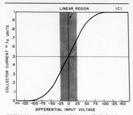
FIGURE 4: Symmetrical characteristic which causes
odd-order distortion.
Here I would like to mention two more typical static characteristics with which you are familiar: crossover non linearity (Fig. 5a) and hard-limiting nonlinearity (Fig. 5b). The crossover nonlinearity is typical of a bipolar or a MOSFET output stage working in Class B. The hard-limiting type is typical for a feedback amplifier after its output stage reaches saturation. Because the slope (gain) of the transfer characteristics is zero in the crossover region in Fig. 5a and in the limiting region in Fig. 5b, feedback is unable to correct such nonlinearities. After all, feedback works on the principle of ‘wasting ’ some of the forward gain of the device in the feedback loop, but if the forward gain is zero, feedback cannot work.
We can correct crossover distortion by circuit design; we bias the output devices into conduction so the forward gain is more than zero. Unfortunately, this does not deal with the hard-limiting type, although we can increase the supply voltage, naturally assuming the devices can take it. The crossover non linearity is famous for producing higher-order harmonics, which results in an unpleasant sound. Although the hard limiting cannot be represented by the third-order truncated power series (equation 3), its qualitative behavior is similar to the series and produces odd-order intermodulation products.
Dynamic Distortion
As mentioned earlier, the coefficients A2, A3, and so on, can also be complex, amplitude and frequency dependent.
When the nonlinearities are both amplitude and frequency dependent, we are talking about dynamic distortion.
Some types have received far too much attention, which, in some cases, has led to questionable design methodologies; whereas others, some at least as important, have been ignored by the design community.
One dynamic type, transient inter modulation distortion (TIM), has received a lot of attention.’ TIM is associated with negative feedback and the unavoidable feedback compensation. Before I embark on a description, note that this problem is not new and TIM-free amplifiers existed long before its ‘invention.’ Also, because it is associated with feedback, many critics demanded feedback-free amplifiers.
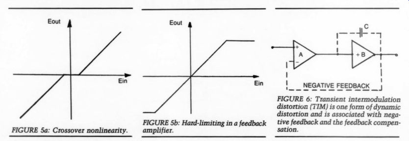
FIGURE 5a: Crossover nonlinearity.
FIGURE 5b: Hard-limiting in a feedback amplifier.
FIGURE 6: Transient intermodulation distortion: (TIM) is one form of dynamic distortion and is associated with negative feedback and the feedback compensation.
Although amps with no global feedback are TIM-free, amps with lots of feed back don’t necessarily suffer from TIM, either.’ Figure 6 shows the block schematic of a typical two-stage audio amplifier, where A represents the input stage (here drawn with differential input for convenience), and B the second stage, which can also include a unity-gain power output stage. If you apply negative feedback around both stages, as indicated by the dotted line, a large portion of the input signal will be canceled by the feedback, leaving a small portion plus the error signal to drive the amplifier. Because of the inherent phase shifts in the amplifier ’s stages, the signal that is fed back to the input will be more and more out of phase with the input and at some high frequency it will reach 180°. The feedback signal at this frequency will cause positive feed back. If the forward gain of the amplifier is still more than unity at this frequency, you have an oscillator. To avoid this, you must roll off the gain to less than unity at this frequency, and you do this with a feedback compensating capacitor.
So far everything is okay. We con front a problem when the input is driven with a fast-rising signal. For the feedback to have 100% control of the amplifier ’s operation, the input stage (A) must charge/discharge the compensation capacitor at the same rate o change as the input signal. This re quires a high current (from A), which it might not be able to supply. If the feedback signal arrives a bit late, during which the input sees a higher than normal input signal, this will produce an overshoot (current or voltage, de pending on the design of the input stage) in the input stage to increase the charging of the capacitor. If the over shoot is large, the input stage (A) might not be able to handle the situation without nonlinearity or straight clip ping. When the overshoots are clipped the amplifier is said to be in slew-rate limiting. This is a hard nonlinearity, and if it is symmetrical it will look like a third-order, but frequency dependent nonlinearity, causing odd-order inter modulation products if at least one o the input frequencies is a high frequency signal.
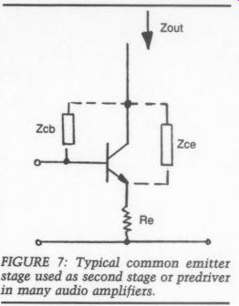
FIGURE 7: Typical common emitter stage used as second stage or predriver
in many audio amplifiers.
To avoid early clipping in the input stage, the amplifier must be designed to handle large input signals under transient conditions. This is equivalent to higher slew rate. You can increase the slew rate by increasing the current ni the input stage, which will charge capacitor C faster. However, just increasing the current will also increase the gain by the same factor, and this will require a larger capacitor to keep the amplifier stable, and you are back to the same slew rate as before. Emitter/source degeneration is one design method used to increase the current without increasing the gain. You can find many articles in the audio press about the necessary size of degeneration to avoid slew-rate limiting, consequently I will not comment on this subject here.
Most modern audio amplifiers boast slew rates in the tens (and hundreds!) of volts/u-sec, which should virtually guarantee against all slewing-induced distortion (SID) caused by hard non linearity. However, you will most likely have TID long before you reach hard clipping in the input stage (A). The soft nonlinearity in the input stage causes sub-slewing TIM. Fortunately, the remedy we mentioned for slew rate also works for the soft nonlinearity. If you recall my explanation about the differential amplifier (TAA 5/83), local emitter/source degeneration also increases the linearity of the transfer characteristics, thus allowing linear operation up to the real slew-rate limit...
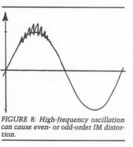
FIGURE 8: High-frequency oscillation can cause even- or odd-order IM distortion.
...of the amplifier. Naturally, designing linear and slew-limit free amplifiers re quires more than using degeneration in the input stage; this description explains only one of the possible forms of dynamic distortion.
Another important form of dynamic distortion in transistor audio amplifiers is caused by transistor junction capacitance nonlinearity. ’ Junction capacitances are a function of the voltage across the junction and capacitances in fluence the open-loop gain at high frequencies, so if you modulate the junction capacitance with the audio signal, distortion will result. The input stage voltage swing of a voltage or power amplifier is usually low, thus the input stage suffers relatively little from this distortion. However, the second stage of just about any amp, especially the predriver stage of a power amp, works with extreme voltage excursions and consequently suffers from junction capacitance nonlinearities.
Figure 7 shows a simplified common emitter (CE) stage used as the second stage in many audio amps. The previously mentioned capacitances are represented here with collector-base impedance Ze and collector-emitter impedance Z.. (Also, the base-emitter capacitance Z. is present, but as long as you drive the stage from a low-impedance source, its influence is negligible.) Again, without mathematical analysis, we can easily see that the output impedance will decrease with in creasing frequency, resulting in decreasing open-loop gain. If you now modulate the junction capacitances with a large audio signal, it will modulate the output impedance as a function of amplitude and frequency, causing dynamic distortion. The solution is to use circuit techniques that make the output impedance very high and independent of the junction capacitances, thus avoiding the modulation effects. I will come back to such techniques in a later article, where I will present some improvements for existing designs and new circuit topologies.
TEST SIGNAL SOURCE THD ANALYZER
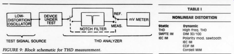
FIGURE 9: Block schematic for THD measurement.
-------------
TABLE 1: NONLINEAR DISTORTION
Dynamic High freq. THD DIM 30/100 Polarity mod. sawtooth IEC IM CCIF IM Cordell MIM THD SMPTE IM IEC IM
---------------
One more form of dynamic distortion we often overlook deserves mention: high frequency oscillation. It appears mostly in power amplifiers, and is usually amplitude and frequency dependent. Assume you are trying to reproduce a 5kHz sine wave and the amp bursts into a high frequency oscillation at the top of the waveform (Fig. 8). The oscillation is neither sinusoidal nor symmetrical. If you remove the high frequency component with a low pass filter, you will find the low frequency (audio) signal has suffered from an even-order, or if the oscillation is symmetrical on both peaks, odd-order, distortion. This oscillation can be caused by junction capacitance modulations, but can also appear in high-speed amplifiers, where unshielded speaker cables feed enough signal back to the input to make them unstable.
Nonlinear Distortion Measurements
From this brief overview of the most important nonlinearities, we can conclude that some sort of measurements are indeed necessary during the design process and also in the evaluation of audio devices. Naturally, this does not exclude listening as part of the design and evaluation process, however, I believe that measurements should always be an integral part of both.
Table 1 shows a summary of the most common measurements used for nonlinear distortion.
Measuring Static Distortion
The most widely used test for static nonlinearities is the 1kHz THD method. Figure 9 shows the block schematic for a THD measurement. A high-purity sine wave is applied to the input of the device under test. The output of the device is fed to the THD analyzer, which consists of a notch filter and an RMS calibrated, average responding millivoltmeter. In principle, the measurement is simple: you adjust the reference level to 100% by by-passing the notch filter, and switching to the measurement position, you remove the fundamental by nulling the notch filter.
The remaining signal consists of the harmonics, which are measured on the millivoltmeter.
The THD is defined as the ratio of the RMS sum of the harmonics and the fundamental. Practical measurements might take time, unless you have a THD analyzer with automatic nulling circuitry. To my knowledge, all commercial THD analyzers have such nulling, making THD measurements easy and fast. Typical measurement limit of THD analyzers is less than 0.002% in the audio band. At low-level THD, noise contributes to the reading and eventually dominates it. These readings are therefore termed THD+N, emphasizing the presence of noise.
Alternatively, you can use a spectrum analyzer instead of the THD analyzer. With this device you can view all harmonics individually, allow you to assess the nature of the nonlinearities. However, this method is expensive and time consuming, because you must add up the harmonics to calculate THD. Also, the measurement floor is limited to 80-90dB, depending on the spectrum analyzer.
Combined with an oscilloscope picture of the harmonic components, the THD analyzer lets you judge the type of nonlinearity dominating the transfer characteristic: square-law producing second harmonics, cubic producing third harmonics. You can use THD to check and adjust crossover distortion, which shows up as spikes in the distortion output. You can check for RF oscillation with different loads (for example, capacitive loads) and over the whole output voltage range; the THD jumps orders of magnitude when oscillation is present. Although the 1kHz THD measurements might not tell you all the truth, the THD analyzer is an important tool in assessing static nonlinearities. I see no point in going further with a design if this test produces unacceptable results.
Another way of exercising static non linearities is to use two tones instead of one, to generate intermodulation products, as described earlier. The oldest IM test is the SMPTE (Society of Motion Picture and Television Engineers) test, which has been used extensively in the recording and film industry because of its inherent insensitivity to wow and flutter. The block schematic of the SMPTE test is shown in Fig. 10a. The test signal consists of a low-frequency tone (f1 = 50-60Hz) and a high-frequency tone (f2 = 6-7kHz), summed in a 4:1 ratio. The low-frequency signal modulates the high-frequency one, and the modulation components appear as side bands around f2 (see Fig. 10b):
even-order, f2 - f1, f2 + f1; odd-order, f2 - 2f1, f2 + 2f1, and so on.
The IM distortion percentage is defined as the RMS-summed side bands referred to the level of the high-frequency tone.
The SMPTE analyzer is quite simple.
First, it removes the low-frequency signal f1, using a high-pass filter. The side bands are then demodulated, using an amplitude modulation (AM) detector.
Finally, the residual carrier components are removed with a low-pass filter.
Because of the analyzer ’s limited band width, the noise floor is very low. The analyzer is not sensitive to the test signal ’s harmonics, so you may use simple oscillators.
For typical transfer characteristics (square law, cubic, and so on), the SMPTE test is approximately 12dB more sensitive than the THD test. It is specifically recommended for excitation of low-frequency, thermally related nonlinearities. It is also quite sensitive to crossover distortion and clipping. For dynamic nonlinearities, the SMPTE test is less predictable. Practical experience shows that audibility of distortion products below 0.5% is poor. ’ The masking effect around the high frequency tone is very high.
A different type of IM test, the IEC IM test (International Electrotechnical Commission), which I have listed under both categories, is a general purpose method of detecting a broad range of nonlinear distortions, both static-and dynamic-within its ability to exercise high-freq non-linearities. In fact, neither this test nor others mentioned later, is able to measure one or the other type of distortion exclusively, unless the test con figuration is well controlled.
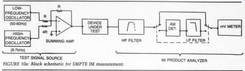
FIGURE 10a: Block schematic for SMPTE IM measurement.
TEST SIGNAL SOURCE IM PRODUCT ANALYZER
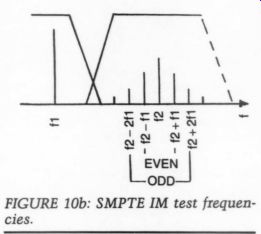
FIGURE 10b: SMPTE IM test frequencies.
In its current proposal, IEC recommends two equal amplitude sine waves with frequencies f1 = 8kHz and f2 = 11.95kHz. Two of the six possible intermodulation products are very close to 4kHz: the second-order, difference frequency product (f2 - f1 = 3.95kHz) and the third-order, difference-frequency product (2f1 - f2 = 4.05kHz).
The IM meter detects these two components. The IEC test is therefore sensitive to both asymmetrical and sym metrical nonlinearities. Since the test signals, as well as the measured distortion products, are all within the audio band, this test is suitable for practically all existing audio equipment, including band-limited devices-tape recorders, PCM digital recorders, transmission lines, and so on.
Dynamic Distortion Measurements
The simplest test for dynamic non linearities is the high-frequency THD test. Walt Jung specifically recommends it for testing IC op amps.! ’ You can also use it for TIM only, but you must control the test configuration completely to avoid other forms of distortion. Jung suggests a unity-gain inverter and the measurement method is to apply a 100Hz signal at full rated output and then sweep the frequency up to 100kHz, noting the 1% point, which indicates the power bandwidth and which coincides with the slew-rate limiting. Naturally, the same measurements can be carried out at lower levels, indicating a correspondingly higher frequency for the dynamic distortion’s Because this measurement requires that the rest of the unit has a closed loop bandwidth of up to 400-500kHz, it is not suitable for band-limited systems, such as a tape recorder. Also, it might prove catastrophic to some power amplifiers, because of output stage stress. Harmonics beyond 20kHz are not audible, and thus have little relevance to the auditory sensation of distortion; nevertheless, this test is valuable in assessing the device ’s linearity and the effect of the feedback at high frequencies.
A single high-frequency THD measurement has also been suggested. A 20kHz sine wave, which has the highest change of rate of the in-band sinusoids (0.125V/usec per volt peak), is able to exercise dynamic nonlinearities, including TIM. Here, at least the input signal is within the audio band, but all the harmonics are still outside. The ad vantage is that it produces a single number, which is easy to understand.
Also, some amps include a THD figure at 20kHz and at rated output/power, so you have a reference to work with.
Although I routinely test all my designs at 20kHz and at different output levels, my main interest with 20kHz testing ...
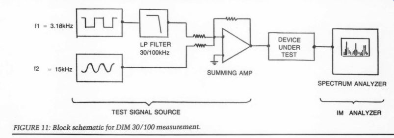
FIGURE 11: Block schematic for DIM 30/100 measurement. IM ANALYZER -- TEST
SIGNAL SOURCE
FIGURE 12a: Block schematic for CCIF IM measurement. IM PRODUCT ANALYZER, TEST SIGNAL SOURCE
... is to look at open-loop linearity, and to test the amp for overload capability and recovery.
The dynamic intermodulation tests DIM-30 and DIM-100 have been developed specifically for testing TIM in audio amplifiers.’’ These tests use a 3.18kHz square wave and a 15kHz sine wave in a 4:1 peak amplitude ratio (Fig. 11). The DIM-30 filters the square wave with a 30kHz LP filter; the DIM-100 with a 100kHz one. All possible IM products are given by the following formula:
Fim,n) = + (m x 3.18kHz) + (n x 15kHz) ... where m and n are integers. Only those with m = 1to9 and n = 1 are defined as DIM products.
The various in-band products are displayed on a spectrum analyzer, and the nine DIM components are summed in an RMS fashion and referred to the 15kHz amplitude to calculate the distortion percentage. The DIM-30 has a rate of change of 0.32V/usec per volt peak and is certainly capable of exercising existing nonlinearities (any and all, mind you, not just TIM, unless you carefully control the test configuration) and produces distortion products.
However, these tests have a number of drawbacks. First, even with the square wave filtered at 30kHz, a large percentage of the test signal slope is contributed by harmonics outside the audio band, which puts an unrealistic burden on an amplifier. Second, the instrumentation is expensive, and its dynamic range is limited-a spectrum analyzer with 80-90dB dynamic range can only measure down to approximately 0.03% distortion. Also, the measurements are quite difficult, you must sum the defined IM products on a CRT screen that locks like a forest.
Finally, some heatedly question the validity of these tests as they relate to auditory sensation of distortion, and no clear criteria have been established so far. This is probably not surprising: the harmonics of the square wave mask al most the entire audio frequency range. ’ A simplified version of this test has also been suggested. It replaces the spectrum analyzer with an analyzer that eliminates all distortion components above 2.4kHz with very steep LP filters and measures only the two IM components that fall below the square wave frequency (900Hz and 2.28kHz).
Proponents report good correlation between the normal DIM measurements and the simplified Skritek method.Takahashi and associates have pro posed a special TIM test using a polarity-modulated saw-tooth. To my knowledge, this test is not widely used and therefore I will not describe it in detail.
As you have seen, both the high frequency THD and the DIM tests rely on out-of-band signals to exercise high frequency nonlinearities. A much more realistic testing of dynamic distortion is to use two- or multi-tone intermodulation tests, where the tests signals are in-band, and the intermodulation products are folded back into the audio band. In other words, inputs and inter mod products are all in-band. The IEC IM test is one method. Two similar methods we are going to look at are the CCIF IM test and the Cordell MIM test.
The CCIF IM test (Commite Consultatif International Telephonique) also uses two equal-amplitude sine waves, but the frequencies are close together and higher: f1= 19kHz and f2 = 20kHz (Fig. 12a). Essentially, all inter modulation tests can detect even- and odd-order distortion products; the question is whether or not the test is looking at both types. The CCIF IM test produces a second-order, difference frequency at f2 - f1 = 1kHz (Fig. 12b), which is the only frequency the test is looking at. However, one of the odd order products: 2f1 - f2 = 18kHz is within the audio band and could be measured with a spectrum analyzer, but again, this requires very expensive instrumentation.
An interesting feature of the CCIF type IM test is that other frequencies, which produce the same difference frequency, can be used. This makes it easily adaptable to band-limited systems with less than 20kHz bandwidth.
We will look at this in Part II. The CCIF test ’s advantage is the IM product is far removed from the input frequencies and thus, outside the auditory masking effects. Therefore it should produce good correlation between test results and auditory sensation. ’ To assess the capability of the CCIF test to detect TIM related distortion, we look at the maximum rate of change of the composite signal.
Assume that the input signal is:
Vin(t)=V1 x sin wlt+V2 xsin w2t (8)
The derivative of this composite signal is:
dVin/dt = (V1 x wl) cos wlt + (V2 x w2) cos w2t (9)
You get the maximum rate of change when cos wlt = cos w2t = 1:
dVin/dt (max) = (V1 xwl)+ (V2 xw2) (10)
The CCIF test uses two equal-amplitude sine waves, so the peak amplitude of the composite signal is twice that of a single sine wave. If we normalize the signal to 1V peak, each frequency will be 0.5V peak. The maximum normalized rate of change will therefore be:
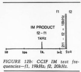
FIGURE 12b: CCIF IM test frequencies-f1, 19kHz; 2, 20kHz.
0.5( omega 1 + omega 2) = 0.5 (19,000 + 20,000) x 2-pi = 0.1225V/usec per volt peak (11)
The rate of change of the CCIF test signal is practically the same as that of the 20kHz THD test signal (0.1256V/ u-sec per volt peak) and is indeed cap able of exercising TIM-related nonlinearities. Naturally, it does not work at all if you are only looking at the difference-frequency and the nonlinearity is purely symmetrical; a rare occurrence, but you must be aware of this, when using the normal CCIF test.
The Cordell multi-tone intermodulation test, or MIM, is similar to the CCIF IM, but by adding a third tone it produces an even- and an odd-order close to each other so they can both be detected simultaneously.
The three test frequencies are:
f1 = 9kHz
f2 = 10.05kHz
f3 = 20kHz
Two produce a difference tone of f2- f1 =1.05kHz, indicating an asymmetrical or even-order nonlinearity; a triple beat, indicating symmetrical or odd-order nonlinearity is produced at f3 - f2 -f1 =950Hz (Fig. 13).
All asymmetrical and symmetrical nonlinearities, not just second- and third-order, are exercised. The IM percentage is ...
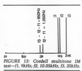
FIGURE 13: Cordell multi-tone IM test-f1, 9kHz; f2, 10.05kHz, f3, 20kHz.
...defined as the two products, measured on an RMS calibrated average-responding millivoltmeter, referred to the RMS value of a sine wave of the same peak to-peak amplitude as the MIM test signal.
The maximum rate of change of the Cordell test signal is less than that of the 20kHz THD or the CCIF. This is due to the two lower frequency components. The maximum rate of change is:
4%(9,000 + 10,050 + 20,000) x 2x 0.08179V/ usec per volt peak In spite of this, the Cordell MIM test has a number of desirable characteristics for general purpose audio measurements: moderately priced instrumentation, simple measurement procedure, good sensitivity to midband even and odd-order intermodulation products, and most importantly, in-band test signals and in-band intermodulation products.
Now that you have the fundamentals of the most used nonlinear distortion measurements, I will describe a two and three-tone intermodulation meter in Part II of my article, with which you can carry out four different IM tests, including CCIF and Cordell. In Part III, I will apply these measurements to a number of existing amplifier designs, and, I hope, by learning from these measurements, I will be able to propose a number of improvements. Several new topologies will also be suggested.
The ultimate test, of course, rests with you: I will ask you to help me evaluate these improvements for sonic quality.
ACKNOWLEDGMENTS
Dr. Kalman Molnar, consultant, reviewed this article and suggested corrections and many excellent improvements. He also put my intuitive mathematical fantasies onto solid ground. I greatly appreciate his contribution.
REFERENCES
1. Lin, H.Y., ‘Measurements of Auditory Distortion with Relation Between Harmonic Distortion and Human Auditory Sensation, ’ IEEE Trans. on Instrumentation and Measurement, Vol. IM-35, No. 2, June 1986.
2. Preis, D., ‘Linear Distortion Measurement Methods and Audible Effects,’ AES Int. Conference, preprint C1005, May 1984.
3. Talbot, D.B., ‘A Review of Nonlinear Distortion Fundamentals,’ AES Convention, preprint 2134, Oct. 1984.
4. Aartsen, G., ‘On the Replacement of THD as the Standard Figure of Merit, ’ AES Convention, preprint 2159, Oct. 1984.
5. Otala, M., ‘Transient Distortion in Transistorized Audio Power Amplifiers, ’ IEEE Trans. on Audio and Electroacoustics, Vol. AU-18, Sept. 1970.
6. Daugherty, D.G. and R.A. Greiner, ‘Some Design Objectives for Audio Amplifiers, ’ IEEE Trans. on Audio and Electroacoustics, Vol. AU-14, No. 1, March 1966.
7. Cordell, R.R., ‘Another View of TIM, ’ Part I and II. Audio, February & March 1980.
8. Cabot, R.C., ‘A Comparison of Non linear Distortion Measurement Methods, ’ AES Convention, preprint 1638, 1980.
9. Stanley, G. and D. McLaughlin, ‘Transient Intermodulation Distortion and Measurement, ’ AES Convention, preprint 1308, 1977.
10. Small, R.H., ‘Total Difference-Frequency Distortion: Practical Measurements, ’ JAES, Vol. 34, No. 6, June 1986.
11. Jung, W.G., et al., ‘An Overview of SID and TIM, Part II: Testing, ’ Audio, July 1979.
12. Leinonen, E., et al., ‘A Method for Measuring Transient Intermodulation Distortion, ’ JAES, Vol. 25, April 1977.
13. Skritek, P., ‘Simplified Measurement of Squarewave/Sine and Related Distortion Test Methods, ’ AES Convention, preprint 2195, 1985.
14. Hofer, B.E., ‘Practical Extended Range DIM Measurements, ’ AES Convention, pre print 2334, March 1986.
15. Takahashi, S., et al., ‘A New Method for the Measurement of Transient Intermodulation Distortion, AES Convention, pre print 1478, 1979.
16. Cordell, R.R., ‘A Fully In-Band Multi tone Test for Transient Intermodulation Distortion, ’ JAES, Vol. 29, No. 9, Sept. 1981.
Also see:
AC SENSING CONTROL, By LB. Dalzell