A knowledge of fundamental mathematics is a necessity for a good understanding of broadcast engineering. A background equivalent to high school mathematics is assumed in this guide. This Section will serve as a review of fundamental relationships and as a reference for the remainder of the text. You can readily determine whether or not you need to study this Section by taking the examination at the end of the Section.
NOTE: Appendix A contains tables of common logarithms, natural trigonometric functions, and decibels.
2-1. NUMBERS
Real numbers when given in simple sign-less form such as 1, 2, 3, 30, etc., are automatically taken as positive values. But we know that it is also necessary to consider zero and negative numbers. See Fig. 2-1A. Zero is a reference or starting point. If we travel 2 miles east (to the right) from this starting point, then turn around and travel 4 miles west (to the left through the starting point), we can express the result as +2-4 =-2 miles.
Be sure to visualize this relationship properly. We traveled in a positive direction for two miles, then turned around. If we had then traveled in a negative direction just two miles, we would have ended our trip at the starting or reference point (zero) , although we had traveled a total of four miles. But we actually continued on through the starting point for a total of four miles in the negative direction, with the end result of arriving at the-2 mile point. This is a total excursion of six miles.
We can just as accurately plot the positive and negative values along the north-south (y) axis as along the east-west (x) axis, as shown in Fig. 2-1B.
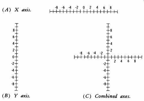
Fig. 2-1. Graphical representation of whole numbers. (B) Y axis. (C) Combined
axes.
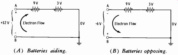
Fig. 2-2. Basic example of negative values. (A) Batteries aiding. (B) Batteries
opposing.
Or we can combine Figs 2-1A and 2-1B to form the pattern of Fig. 2-1C.
The directions of positive and negative values illustrated are those conventionally used.
The real number system consists of:
Zero (starting point) Whole numbers (positive or negative)
Rational numbers (expressed as whole numbers or fractions)
Irrational numbers (which cannot be expressed as simple fractions) An example of an irrational number is the square root of 2 (\). This cannot be expressed as a simple fraction.
Whole numbers are also called "integral numbers." These are termed "even numbers" when exactly divisible by 2. When not exactly divisible by 2, they are called "odd numbers."
Adding and Subtracting Positive and Negative Numbers
Fig. 2-2 illustrates a basic electronic example of negative values. In Fig. 2-2A, a 3-volt and a 9-volt battery are connected in series aiding. A volt-meter between points A and B shows point A to be 12 volts positive relative to reference (zero) point B (9 + 3 = 12) . It is just as accurate to say that point B is 12 volts negative relative to point A. In Fig. 2-1B, the 9-volt battery has been reversed. Now the voltmeter shows point A is 6 volts negative relative to reference point B (-9 + 3 =-6 volts) . Or we can say that point B is 6 volts positive relative to point A. If we place a resistor between A and B in each circuit, the direction of electron flow between the terminals is in opposite directions in the two circuits.
Thus we have illustrated the basic rule of addition of positive and negative numbers. When we add two numbers of unlike sign, we simply sub tract the smaller number from the larger number, and place the sign of the larger in front of the answer. When more than two numbers of unlike signs are to be added:
1. Add all positive numbers.
2. Add all negative numbers.
3. Subtract the smaller sum from the larger sum and affix the sign of the larger to the answer.
For example, add-2, 4,-8, 6,
Solution:
9.
-2 4
-8 6 9
-10 +19 so:
19+ (-10) =+9
When adding only negative numbers, simply add all the numbers and affix the negative sign to the sum.
Now let us return momentarily to the travel example used in conjunction with Fig. 2-1A. In that example, we traveled a total of 6 miles and ended at the-2-mile point relative to the starting point. Now suppose we turn around again and travel 2 miles east. We arrive at our starting point (zero) . What we have done essentially is to subtract - 2 miles from our trip, which was exactly equivalent to adding a positive 2.
Thus, subtracting a negative number is equivalent to adding a positive number. The rule in subtraction is to change the sign of the subtrahend and add. For example, to subtract-10 from 6:
6 Minuend
-10 Subtrahend (Change sign to +.) 16 Remainder
This would be expressed in equation form as:
6-(-10) = 16
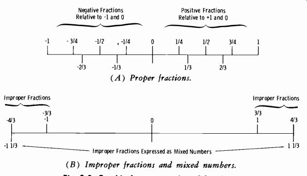
Fig. 2-3. Graphical representation of fractions.
(A) Proper fractions. Improper Fractions Expressed as Mixed Numbers (B) Improper fractions and mixed numbers.
Fractions
Fig. 2-3 is a basic graphical representation of fractions. Proper fractions (values less than 1) are shown in Fig. 2-3A. Improper fractions (those totaling 1 or greater) are shown ,in Fig. 2-3B, which also indicates that improper fractions can be expressed as mixed numbers containing a whole number and a fraction.
The top number of a fraction is termed the numerator. This is an indicator of the number of fractional parts expressed. The bottom number of a fraction is termed the denominator. This is an indicator of the number of parts into which the whole unit has been divided.
Observe from Fig. 2-3A that smaller values are always to the left of 0 (the starting point) and larger values are always to the right of the starting point. The fraction - 1 1/4 is larger than the fraction -1/2 because it lies to the right, as shown graphically. Conversely, the fraction 1/2 is larger than the fraction VI, again because it lies to the right on the graph.
Before we go further, note that the product (result of multiplication) can be written as (for example) 2 x 6 = 12 with the conventional multiplication sign. It can also be written (2) (6) = 12. We will use the latter form in this text.
The following basic rules for fractions apply:
1. The numerator and denominator can be multiplied or divided by the same number without changing the value of the fraction.
For example, multiplying both the numerator and denominator of the fraction 3/3 by 2 gives:
(2) (2) _4 (3)(2) 6
... which is equivalent to 33.
Or, taking 4/6 and dividing both numerator and denominator by 2 gives:
4/2_2 6/2 3
2. To multiply a fraction by a given number, the numerator is multi plied by the number, or the denominator is divided by the number.
For example,
4(2)=(4)(2) 8 =-1 1/3 6 6 6 or 4 _4=1 1/3 6/2 3
3. To divide a fraction by a given number, the numerator is divided by the number, or the denominator is multiplied by the number.
For example, 4/6 divided by 2:
4/2_2_1 6 6 3 or 4 _4_1 (6)(2) 12-3-
4. To add fractions:
(A) Convert all the fractions to the lowest common denominator.
(B) Add all the numerators.
(C) Put that sum over the denominator.
For example: 1/6 + 1 1/4 + 1 1/2 To find the lowest common denominator (LCD) , find the smallest number into which each denominator can be divided a whole number of times. In this example, 6 will go into 12 2 times, 4 will go into 12 3 times, and 2 will go into 12 6 times. Therefore 12 is the lowest common denominator.
Since 6 goes into 12 twice, then 1/6 is the same as 2/12. Since 4 goes into 12 3 times, 1/4 = 3/12. Since 2 goes into 12 6 times, 1/2=6/12. Then:
12 + 12 + 12 = 12
In the above example, the lowest common denominator was easy to find just by observation. Sometimes this is not the case; consider 1/5 + 1/4 + 1/2.
To find this LCD, we use factoring. This simply means reducing to fundamental quantities. Since 5 and 1 are the only whole numbers that can be multiplied together to give 5, 5 is not factorable. Similarly, 2 is not factorable. But 4 = (2) (2) . So we have:
5=5 4= (2) (2)
The number 2 appears twice in 4, so (2) (2) must be a part of the LCD, which must also include a 5. Thus:
LCD = (2)(2)(5)=20
Then changing the fractions to the LCD:
1/5 = 4/20 1/4=5/20 1/2 = 10/20
Thus:
4 5 10 _ 19 20 + 20 + 20 20
5. To convert a fraction to a decimal number, divide the denominator into the numerator. In the preceding example, the sum 4/20 + 5/20 4- 10/20 was found. These fractions can be converted to decimals as follows: 4/20 = 0.2, 5/20 = 0.25, and 10/20 = 0.5.
Then:
0.20
0.25
0.50
0.95 total
This total stated in fractional form is ninety-five one-hundredths (95/100). Dividing both numerator and denominator by 5 gives 19/20, which was the answer obtained under rule 4 above.
6. To subtract one fraction from another fraction, (A) change both fractions to the same denominator as in rule 4 for addition, (B) sub tract one numerator from the other numerator, and (C) place the remainder over the denominator. For example:
1 1_5_4_1 4 5 20 20 20
7. To multiply fractions, multiply the numerators and then multiply the denominators. For example, (1/4) (1/5) = 1/20. The product of fractions always is less than either of the fractions. Take another example: (3/5) (3/6) = 9/30. Note that 9/30 can be reduced to 3/10 by dividing both numerator and denominator by 3.
8. To divide fractions, invert the divisor and then multiply. To keep your perspective on this rule, note that (for example) multiplying a number by 1/5 is the same as dividing that number by 5. Thus (3) (1/5) = 3/5. Note that this is the same as dividing three by five (3/5).
For example, if 2/5 is to be divided by 3/7:
5 7-(5) (3) 15 Note that the divisor, 3/7, was inverted (7/3), and then the multiplication rule was used.
9. When a series of different operations must be performed, do them in the following sequence:
1. Multiplications.
2. Divisions.
3. Additions.
4. Subtractions.
For example, solve 24-6- (4)(10) +5+ (20) (3)-2
Multiplications: 24 ± 6- 40- 5 + 60-2
Divisions: 4-8 + 60-2
Additions: 64-8-2 Subtractions: 64- 10 = 54 (Answer) 2-2.
PERCENTAGE
A percentage is a fractional value having a denominator of 100. For example, 1 percent is the same as 1/100 or 0.01, 6 percent is the same as 6/100 or 0.06, and 75 percent is the same as 75/100 or 0.75.
If a power supply is said to be regulated within 1 percent of 280 volts, what is the allowable departure from 280 volts? Since 1 percent = 0.01, then (280) (0.01) = 2.8 volts (answer) .
The regulation of a power supply is often computed in terms of the voltage difference between no-load and full-load conditions:
% Regulation =E1-E2 (100) where, E1 is the no-load voltage, E2 is the full-load voltage.
For example, if El = 300 V and E2 = 290 V, then:
300- 290
% Regulation =
290 (100) 10 290 (100 )
= (0.0344) (100) = 3.44%
2-3. EXPONENTS AND SQUARE ROOTS
The exponent of a number is a small figure placed at the upper right of the number. For example, 10^2 means that the number 10 is used as a factor two times, thus:
10^2 = (10)(10) = 100
Similarly,
10^3= (10)(10)(10) = 1000
When the exponent is positive as in the above examples, the result is greater than unity, if the number being multiplied is greater than unity.
The expression 10^2 is to the power 2; 10^3 is read "ten raised to the third power"; etc.
When the exponent is negative, the reciprocal of the number (the number divided into 1) is raised to a positive power. Thus:
10 '=1-(10) (10) (10) (10) 10,0100-0.0001
When the exponent is negative, the result is between zero and unity if the number to be raised to the power is greater than unity.
Unity (in terms of exponents) is any number raised to the zero power.
Thus 10^0 = 1, 2° = 1, etc.
Addition of Exponents
Exponents are added in obtaining the product of like numbers raised to the same or different powers. Thus:
(22) (23) =22+3=23
Or (33) (3°) =33+6=39
When unlike numbers are raised to powers and the product must be found, each number must be raised to the indicated power before multiplication. Thus the product of 22 and 34 is:
(22) (34) = (2)(2)(3)(3)(3)(3) = (4) (81) =324
Subtraction of Exponents
Exponents are subtracted in the division of numbers raised to powers.
Thus:
Or Or
But note that
24 =24 2=22=4 4' 42 3 4-1 4 3 106 lol, 10-y 23_23_3_26_1 2s
(Any number raised to the zero power is equal to unity, or 1).
Multiplication of Exponents
Exponents are multiplied to find the power of a power. Thus (33) 3 = 3s, (33)-3, 3-9, (3-3)2, 3-6, (4-3)-4,412, etc.
Power of a Fraction When a fraction is raised to a power, it can be written as the power of the numerator divided by the power of the denominator. For example:
1 2 12
2) 22 4
Roots
If the power of a number is a fraction, it can be written as the root of the number. Thus 16 1/2 = = 4. The symbol / is always assumed to indicate the square root of the number, and the 2 is omitted. For any other root (such as the cube root, or V-) the order of the root (in this case 3) must be given. The symbol √ is called the radical sign, and the number under the radical is called the radicand.
Extracting Square Root
Extracting the square root of a number is relatively simple compared to extracting higher roots. These roots are obtained by using logarithms, as covered in Section 2-5.
How to extract the square root of a whole number is shown most easily by an example. Suppose it is desired to extract the square root of 48,400.
Proceed as follows.
Step 1. Starting at the decimal point, divide the number into two-digit groups moving to the left: 4'84'00. Note that when the number of digits is an odd number, the leftmost digit is by itself.
Step 2. Find the largest number that when squared (multiplied by itself) will be less than or equal to the first group, in this case the single digit 4.
Since 2 times 2 is 4, place the figure 2 immediately above the 4:
2 V4'84'00
Step 3. The square of 2 is 4, so place this number under the first digit, and subtract:
2 V4'84'00 4
0 Step 4. Bring the second group down with the remainder:
2
\/4'84'00 4 84
(Note that 4-4 is zero, so this is discarded, leaving 84) .
Step 5. Double the number in the answer thus far and bring down the result as the first digit in a trial divisor for 84:
2
\/4'84'00 4 4 )
84 Step 6.
The second digit for this trial divisor must be such that if the total number making up the trial divisor is multiplied by the second digit, the product will be less than or equal to the remainder, in this case 84. We know that the trial divisor will become a number greater than 40 when a second digit is added. Thus 42 is the number, since 42 times 2 (the number added) is exactly equal to 84. So:
2 2 0 (answer) V4'84'00 4 42) 84 84
00'00
Thus in this example, the number added to 40 is 2, and 2 times 42 is 84.
The number 2 is placed immediately above the '84, and since the remainder of the total number is 00'00, a zero (0) is placed immediately above the '00 under the radical sign.
In the above example, we extracted the square root of a perfect square.
In the following example, the radicand is not a perfect square.
Problem: Extract the square root of 1410.
3 7. 5 V14'10.00 9 67 ) 510 469 745) 4100 3725 375
The answer to the first decimal place is 37.5 with a remainder of 375. For greater accuracy (more decimal places) , two more zeros would be brought down and the process continued.
The process is exactly the same in extracting the square root of a number less than unity. For example, find the square root of 0.00026. First, mark off the number in two-digit groups:
.00'02'60
Note that an extra cipher is added to the last digit to make a group of two.
. 0 1 6 1
/00'02'60'00 1 26) 160 156 321) 400 321 79
The answer to four places is 0.0161 with a remainder of 79.
To prove the answer, (0.0161) (0.0161) = 0.000259, or very nearly 0.00026.
Chart 2-1. Powers of Ten
2-4. SCIENTIFIC NOTATION
Scientific notation greatly simplifies computations that involve very large numbers. The process is simpler than would appear from a statement of the basic rule, which is: "Any number expressed in scientific notation is written as a decimal number between one and ten, multiplied by ten raised to the proper power."
Example 1: 5,000,000 = (5) (10^6 )
Example 2: 525 = (5.25) (10^2)
Example 3: 0.000005 = (5) (10^-6)
Example 4: 0.00000024 = (2.4) (10^-7)
These examples illustrate that the decimal point is shifted as many places as necessary, and this result is multiplied by ten raised to a power equal to the number of places the decimal point was shifted. If the decimal point is moved to the left, the power of ten is positive. If the decimal point is moved to the right, the power of ten is negative.
Powers of ten from 10^6 to 10^-6 and the conventional terminology are shown in Chart 2-1.Prefixes commonly used in electronics, along with their symbols and power-of-ten multipliers, are listed in Table 2-1.
In practice, the number need not be reduced to a quantity between one and ten if it is more convenient to do otherwise. In Example 1 above, the result could just as correctly be written as (50) (105). Example 4 could just as accurately be written as (2^4) (10^-8), etc.
Adding and Subtracting Powers of Ten
To add or subtract numbers expressed in powers of ten, simply convert all numbers to the same power of 10, and keep this same power of 10 in the answer.
Table 2-1. Prefix Symbols
Example 1: 3.28 (103) + 1.14 + 12.5(102) 3.28(1W) = 3.28000(103) 1.14 =0.00114(103) 12.5(102) =1.25000(103)
Total =4.53114(103)
Example 2: 3.28 (103)- 1.14(102) 3.28(103) = 32.80(102) 1.14(102) _- 1.14(102) Total = 31.66(102)
Multiplying Powers of Ten
To find the product of numbers when expressed as powers of 10, simply multiply the numbers and add the exponents of the tens. For example:
6.28(103) x 3.14(102) =19.7192(103+2) =19.7192(10b)
For negative exponents:
6.28(10-3) x 3.14(10-2) = 19.7192( 10-2-3) = 19.7192(10-s) For exponents with opposite signs:
6.28(103) x 3.14(10-2) =19.7192(103-2) =19.7192(10) =197.192
Dividing Powers of Ten
To divide numbers expressed as powers of 10, simply divide the numbers and subtract the exponent of the denominator from the exponent of the numerator. For example:
6.28(103)
=2(103-2)=2(10) =20 3.14(102)
Sometimes it is more convenient to transfer the ten in the denominator to the numerator and change its sign:
6.28(103)(10-2) 2(103-2) =2(10) =20 3.14
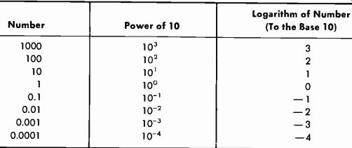
Table 2-2. Integral Powers of Ten
2-5. LOGARITHMS
Logarithms (often called "logs") enable us to simplify complex computations involving multiplication, division, powers, and roots. Logarithms reduce multiplication to a simple addition and division to a simple subtraction; raising to a power becomes a single multiplication, and extracting a root becomes a single division.
There are two generally used systems of logarithms, the common logarithm (most widely used and reviewed in this Section) and the natural logarithm (not covered in this text) . A natural logarithm is indicated by the notation loge, which designates a logarithmic base of 2.718. The common logarithm has a base of 10. The approximate relationship of the two systems is as follows:
Log10 (common log) = 0.4343 times natural logarithm of number
logE (natural log) = 2.3026 times common logarithm of number
The designation log10 is normally written simply as log, the base ten being assumed. Thus log 645 means the common logarithm of the number 645.
The common logarithm of any number is simply the power to which 10 must be raised to equal that number. For numbers that are integral powers of 10, the relationship is extremely simple, as evidenced by Table 2-2.
When the number is not an integral power of 10, the log of that number consists of a whole number and a decimal fraction. The whole-number part of the logarithm is termed the characteristic, and the decimal-fraction part is termed the mantissa.
The Characteristic
Table 2-2 actually lists the characteristic of the number in the column headed "Logarithm of Number." This may be expanded as shown by Table 2-3. Note that the characteristic of a whole number has a positive value equal to one less than the number of digits before the decimal point, and the characteristic of a decimal fraction has a negative value equal to one more than the number of zeros after the decimal point.
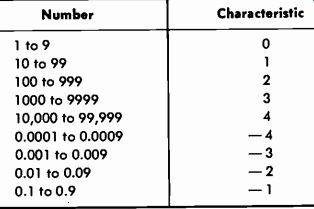
Table 2-3. Characteristics of Numbers
The Mantissa
The decimal-fraction part of a logarithm (the mantissa) is obtained from a table of common logarithms such as Table A-1 in Appendix A.
To find the mantissa in the table, look under the left-hand column (N) and locate the first two digits of the number. Then in the column under the third digit of the number, the mantissa is given. For example, take the number 246. Locate 24 in column N. Then go across to the column numbered 6 and find the mantissa, 0.3909, which will be the decimal part of the logarithm of 246.
Suppose the number is a four-digit number such as 2468. You have already found the mantissa for 2460, which was 0.3909. To find the mantissa for 2468, use the proportional parts column to find the proportional part for 8. This is 14, so the mantissa is 0.3909 plus 0.0014, or 0.3923.
The Combined Characteristic and Mantissa (Logarithm of a Number)
The mantissa is always positive and determines the sequence of digits.
It is the only value given by the log table. The characteristic may be either positive or negative; it determines the position of the decimal point.
You already know that the characteristic is one less than the number of digits to the left of the decimal point. Thus the log of 2468 = 3.3923.
Now suppose you need to find the log of 0.02468. Again, look under the left-hand column (N) to locate the first two digits (24) . Then in the column under the third digit of the number (6) , read 3909. Then again using the proportional-parts column for 8, obtain the same mantissa as before, 0.3923. But now the characteristic is a negative 2. The negative characteristic is equal to the number of digits to the right of the decimal point to and including the first significant digit.
The preceding result could be written 0.3923- 2, but this form is impractical to use. Therefore, convert the characteristic to a positive number, for example: 8.3923 - 10. This is to say that you add 10 (or a multiple thereof) to the negative characteristic, and compensate by indicating the subtraction of 10 from the entire logarithm.
Examples:
Log 0.002468 = 7.3923- 10
Log 0.2468 = 9.3923 – 10
Log 2.468 = 0.3923
Log 24.68 = 1.3923
Antilogarithms
In practical problems it is necessary to find the antilogarithm (often called the "antilog") , which is the number corresponding to a given logarithm. Finding this number is the reverse of finding the logarithm. For example, since the log of 2468 is 3.3923, the antilog of 3.3923 is 2468.
To find the antilog of a number, locate the mantissa in the log table and write it down. Then place the decimal as indicated by the characteristic.
For example, to find the antilog of 3.5453, first look up the mantissa (5453) to find the corresponding number, which is 351. A characteristic of 3 means that there will be 4 digits in the number, or 3510. So antilog 3.5453 = 3510.
Examples:
Antilog 2.5453 = 351
Antilog 1.5453 = 35.1
Antilog 0.5453 = 3.51
Antilog 7.5453- 10 = 0.00351
When you must find the antilogarithm of a logarithm the mantissa of which is not given exactly in the table, proceed as follows:
Step 1. Compute the tabular difference between the next higher and next lower mantissas.
Step 2. Compute the difference between the given mantissa and the next lower mantissa, and divide this figure by the result of Step 1.
Step 3. Add the result of Step 2 to the significant figures corresponding to the next lower mantissa.
Step.4. Place the decimal as indicated by the given characteristic.
As an example, to find the antilog of 2.7376:
Step 1. Next higher mantissa 0.7380
Next lower mantissa 0.7372
Tabular difference 0.0008
Step 2. Given mantissa 0.7376
Next lower mantissa 0.7372
Tabular difference 0.0004
Then:
0.0004 = 0.5
0.0008
Step 3. The significant figures corresponding to the next lower mantissa (0.7372) are 546. To this number, add the result of Step 2, giving 546.5.
Step 4. Since the given characteristic is 2, the antilog of 2.7376 is 546.5.
If the antilog of 3.7376 is to be found, the result is 5465, etc.
To Multiply
To multiply numbers by the use of logarithms, add the logarithms and find the antilog of the sum.
Example 1: Multiply 246 by 788.
Log 246 = 2.3909 Log 788 = 2.8965
Sum = 5.2874
Antilog 5.2874 = 193,848
Example 2: Find (0.03) (0.05) (0.5) .
Log 0.03 = 8.4771 – 10
Log 0.05 = 8.6990 – 10
Log 0.5 = 9.6990 – 10
Sum =26.8751-30
Antilog (26.8751- 30) = 0.00075
To Divide
To divide numbers by the use of logarithms, subtract the log of the divisor from the log of the dividend, and find the antilog of the difference.
Example: Divide 40,500 by 15.4.
Log 40,500 = 4.6075
-Log 15.4 =-1.1875
Difference = 3.4200
Antilog 3.4200 = 2630
Powers
To raise a given number to any power, multiply the log of the given number by the power which the number is to be raised. Then find the antilog of the product.
Example: Find 26.43.
Log 26.4 = 1.4216 x3
Product = 4.2648
Antilog 4.2648 = 18,400
NOTE: The answer 18,400 is as accurate as can be obtained with a four place log table and is normally sufficiently accurate in practice. The actual value of 26.43 is 18,399.744. Six-place log tables are available for use when extreme accuracy is required.
Roots
To find a root of a number by the use of logarithms, divide the log of the given number by the index of the root, and find the antilog of the quotient.
X2.09.
Log 2.09 = 0.3201
0.3201=3=0.1067
Antilog 0.1067 = 1.279 2-6.
ALGEBRA
Ir. ordinary arithmetic, numbers are given in equations. In algebra, letters are used basically to express general conditions. Let us express certain of the Preceding logarithmic relationships in algebraic form as an example:
Log (a) (b) =loga+logb Logb=loga –logb
A basic tool in algebra is the ability to change an expression from one form to another more suitable for the problem at hand. The basic rules are:
if A = B/C, then B = AC, and C = B/A.
Thus when we consider the basic rule of Ohm's law that states that voltage is equal to the product of amperes and ohms (E = IR), we know that I = E/R and that R = E/I.
Another type of expression is the ratio or proportion:
A_C B D
which is read "A is to B as C is to D." Cross multiplying gives AD = BC, and from this:
_ BC AD AD BC A D' B C' C B ' D
A basic formula for tuned circuits is:
1 f= 2TrVLC
This formula (relationship) is true for resonance no matter what numerical values are involved. Thus if you know the two values ( inductance L and capacitance C) , you can compute the frequency of circuit resonance.
But suppose you have a given capacitance and must compute the value of inductance required to resonate with that capacitance at a given frequency. In this case, the two known values are the frequency and capacitance, and the inductance must be found.
First remove the radical by squaring both sides of the equation:
Then solve for L:
f2 = 1 4Ir2LC 1 L 4 pi 2f2C
If the inductance is known and the capacitance is unknown, the formula becomes:
C= 1 4ir-f2L The basic relationship for ac impedance is:
Z = VR2 + X2 where the reactance (X) is actually XL- Xe.
Then Z2 = R2 + X2 and and R=VZ2-X2 X=VZ2-R2
2-7. GEOMETRY AND TRIGONOMETRY
We will make here a basic distinction between geometry and trigonometry that is most important to the electronic engineer. The most valuable use of geometry for our purpose in this text is to find the hypotenuse of a right triangle when the dimensions of the two legs are known. As used in this text, trigonometry is a tool for determining the angles of a right tri angle and their relationship to the sides of the triangle.
In Fig. 2-4A, a force (A) of a 3 units acts at right angles to a force (B) of 4 units. Since there is a difference in direction between the two forces, we cannot add them either arithmetically or algebraically. The solution (the magnitude of the resultant force) must be obtained by geometric addition.
Fig. 2-4B is the graphical representation of completing the rectangle so that the geometric sum of A and B can be represented. Obviously, this sum (C) is simply the hypotenuse of a right triangle. Fig. 2-4C illustrates the conventional representation.
RULE: The hypotenuse of a right triangle is equal to the square root of the sum of the squares of the other two sides.
(A) Forces A and B. (B) Completing rectangle. (C) Geometric addition.
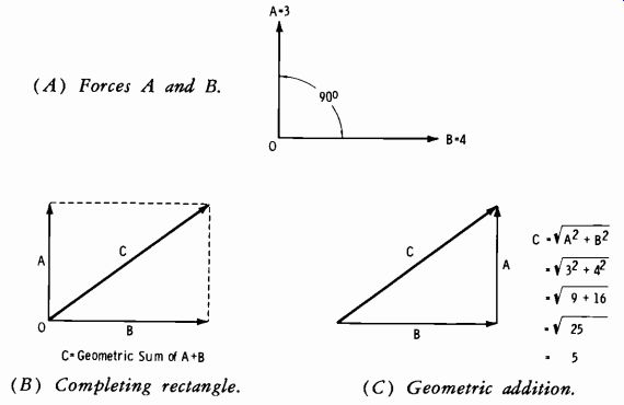
Fig. 2-4. Resultant of two forces at right angles.
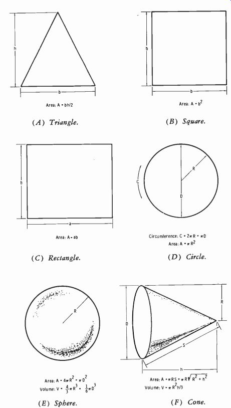
Fig. 2-5. Basic geometric relationships.
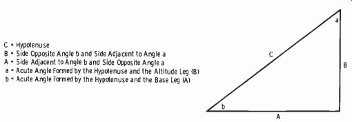
Fig. 2-6. Terminology applicable to trigonometric functions.
C Hypotenuse B Side Opposite Angle b and Side Adjacent to Angle a A Side Adjacent to Angle b and Side Opposite Angle a a Acute Angle Formed by the Hypotenuse and the Altitude Leg (B) b Acute Angle Formed by the Hypotenuse and the Base Leg (A)
Table 2-4. Trigonometric Formulas-----------
The expression "arc sin" or "sin-1" indicates "the angle whose sine is. . .
Similarly, "arc tan" or "tan-1" indicates "the angle whose tangent is ..." , etc.
Thus the resultant of forces A and B in Fig. 2-4 is 5, as indicated in Fig. 2-4C. Note that this solution gives the answer in magnitude only; the angle of the resultant force is determined by trigonometric methods. If the two sides are equal, the hypotenuse forms an angle of 45° with either leg (half way between the two legs). Since force B in Fig. 2-4 is greater than force A, the resultant lies closer to the larger force, B. Hypotenuse C is a vector.
Vector analysis (Section 2-8) uses both geometry and trigonometry.
Fig. 2-5 illustrates additional basic geometric relationships useful to the electronic engineer.
Fig. 2-6 illustrates some of the terminology used with trigonometric cot = opposite side Angles can be formed in any of the four quadrants that make up a complete circle, or 360°. In trigonometric tables, only angles up to 90° are given. Thus the circle is divided into four 90° quadrants as shown by Fig. 2-7. For an angle between 90° and 180°, the trigonometric function is equal in magnitude to the same function of an angle equal to 180° minus the angle in question. This angle will then be between 0 and 90° (that is, the angle is measured from the x-axis) . For an angle in the third quadrant subtract 180°, and in the fourth quadrant subtract the angle from 360°.
In any case, the result is an angle between 0 and 90°.
Assume in Fig. 2-6 that A = 4 and B = 3. What is the magnitude of C, and what angle does it make with the x-axis? From geometry, we know that cos =
hypotenuse tan = opposite side adjacent side adjacent side functions. Table 2-4 applies to this figure. Table A-2 in Appendix A gives the natural sines, cosines, tangents, and cotangents of angles.
NOTE ON USE OF TABLE OF TRIGONOMETRIC FUNCTIONS:
To find values for angles from 0° to 45°, use the headings at the top of the table and the degree listings in the left-hand column. For angles from 45° to 90°, use the headings at the bottom of the table and the degree listings in the right-hand column. Read the degree listings in the right-hand column from bottom to top; thus the 10' listing directly above 89° signifies 89° 10'.
The trigonometric functions of an angle are normally abbreviated as follows:
Sine = sin
Cosine = cos
Tangent = tan
Cotangent = cot
The basic relationships are:
sin =
opposite side hypotenuse adjacent side C=x/42+32= =5
This result gives the magnitude of C but does not specify angle b.
From trigonometry, we know that we can find angle b by any or all of the relationships listed above (sine, cosine, tangent, or cotangent) .
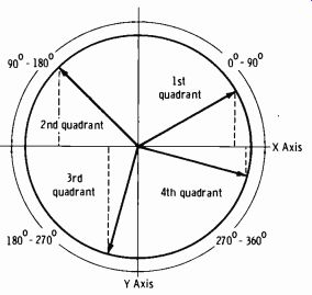
Fig. 2-7. Quadrants of a circle.
Sin b=5 =0.60
Then b = 36° 50' (from trig table by reading to the nearest listed, which is 0.5995) .
cos b = = 0.80 sine value
Then b = 36° 50' ( from trig table to nearest listed cosine value, or 0.8004) tan b =- = 0.75
Then b = 36° 50' (from trig table to nearest listed
0.7490). (The 36° 50' is read "36 degrees, 50 minutes.
The sum of the interior angles of a triangle is 180°.
of angles a and b in Fig. 2-6 is 90°.
When angle b is angle a is found by subtracting angle b from 90°. In-(36° 50') =53° 10'.
Note that if any one angle and one side are known, hypotenuse) can be found by the use of algebra on the given above. Thus, for example, since opposite side sin = hypotenuse then hypotenuse-opposite side sin tangent value, or
Therefore the sum known (36° 50') , this example, 90° the other side (or angle relationships or opposite side = (sin) ( hypotenuse)
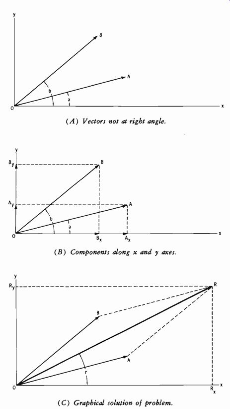
Fig. 2-8. Basic vector addition.
(A) Vectors not at right angle. (B) Components along x and y axes. (C) Graphical solution of problem.
2-8. VECTORS
We have been using vectors in geometry and trigonometry. It is now possible to review vectors in greater detail. Fig. 2-8A shows vectors ( A and B) which are not at right angles. These vectors may be resolved into their components along the x and y axes as illustrated in Fig. 2-8B. Then:
Sum of x components = R. = Ax + Bx
Sum of y components = Ry = AS + B,
The geometric sum of the resultant x and y components (Rx and Ry) yields the resultant vector R at an angle r with the x axis. This is shown in Fig. 2-8C, which illustrates the graphical solution to this problem. Line AR is drawn parallel to vector B, and line BR is drawn parallel to vector A.
The intersection determines the magnitude of resultant vector R.
To solve on paper without drawing a graph, the magnitude of the result ant is:
or actually R=_ /Rx2+Ry2 R=V(Ax+Bx)2+ (Ay+By)
As an example, assume:
A = 8 and angle a = 20° (written 8 / 20° ) B = 6 and angle b = 40° ( written 6 / 40° )
From the fundamental trigonometric relationships:
Similarly, Ax cos a=A Ax=A cos a sin a=A Ay=A sin a
Therefore A,=A cos 20°=8(0.9397) =7.5 A,- = A sin 20 °= 8( 0.3420 ) = 2.7 Then finding the x and y components of vector B:
B,=B cos b=6 cos 40° =6(0.7660) =4.6 B,.=B sin b=6 sin 40° = 6(0.6428) = 3.9
Collecting the x and y components:
R=x/(7.5+4.6)2+ (2.7+3.9)2= 190= 13.8
Note from the above that Rx = 7.5 + 4.6 = 12.1 and that Ry = 2.7 + 3.9
= 6.6.
Therefore tan r = RX = 6.6 = 0.545 then r = 28 ° 40' (approx)
Thus the complete solution is written:
R=13.8 /28°40'
You can find the magnitude of vector R directly in terms of the magnitudes of vectors A and B and trigonometric functions of angles a and b by the following relationship:
R=\/(Acosa + Bcosb)2+ (A sin a+Bsinb)2
Then value of tan r is A sin a + B sin b tan r =
A cos a + B cos b Now see Fig. 2-9.
Given the magnitudes and angles of vectors A and B, find R and angle r.
R = V(8 cos 20° + 20 cos 120°)2+ (8 sin 20°+20 sin 120°)2
Since vector B is in the second quadrant, find the angle it makes with the negative x axis and attach the correct sign:
cos 120° =-cos (180- 120) =-cos 60° then:
R=V/[8(0.9397) +20(-0.5)]2+[8(0.3420) +20(0.866)]2
= V[7.52 + (-10)]2+ {2.74 + 17.32)2
=\/(-2.48)2+ (20)2
=\/6.15+400=\%406=20.1
The magnitude of R is thus 20.1. The tangent of angle r is:
tan r-2 = =-8.06 and the corresponding angle from the table is approximately 82° 55'. But angle r is in the second quadrant, and the angle found in the table is the angle between R and the negative x axis. Angler is then 180°- (82° 55'), or 97° 05'.
The solution to the problem is therefore R = 20.1 / 97° 05'.
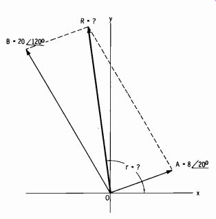
Fig. 2-9. Example of vector addition with vectors in first and second quadrants.
2-9. COMPLEX NOTATION (OPERATOR j)
In the study and measurement of propagation factors and broadcast antennas, it is necessary to understand the combined effect of magnitude and phase. This is most conveniently visualized in vector form. The length of a vector represents the magnitude, and the direction (with respect to a reference axis) represents the phase. The combined result may then be represented by one resultant line.
For example, a circuit employs a resistance of 3 ohms and a coil with inductive reactance (at the frequency specified) of 4 ohms. From fundamental theory, the impedance (Z) is the square root of the sum of the resistance squared and the reactance squared:
Z=vR2±X2=V9+ 16= 25 =5 ohms
While this gives the total impedance, it does not express the resultant phase angle of the total impedance relative to a purely resistive circuit. It is this phase angle that must be considered in the proper phasing and tuning of antenna systems. .
There are two basic notations for expressing a vector quantity. These are the polar form (just described in Section 2-8) and the rectangular form (to be explored in this section) . The rectangular form involving the j operator is a simple expression for impedance that shows the resistive and reactive components directly. In the example of 3 ohms resistance and 4 ohms inductive reactance, the rectangular form is simply 3 + j4.
Inductance is considered a positive reactance; thus it is represented as 4 units up along they axis (Fig. 2-10) . If the reactance is capacitive (negative reactance), the four units are taken down along the y axis, and the rectangular form is 3- j4. The resistance of 3 ohms is represented as 3 units along the x axis.
The +j operator produces 90° counterclockwise rotation of any vector to which it is applied, without changing the magnitude of that vector. The -j operator produces 90° clockwise rotation of any vector to which it is applied, without changing the magnitude of that vector. Successive applications of the +j operator to a vector produce 90° steps in sequence in the counterclockwise direction. Similarly, successive applications of the-j operator to a vector move that vector 90° clockwise for each application.
This is tabulated in Table 2-5.
The addition of quantities in rectangular form is illustrated by the following examples:
Example 1: Add 3 + j4 to 3- j4 3-j4 3 + j4 6- 0
Example 2: Add 3 + j4 to 3 + j4 3+j4 3 + j4 6+ j8
One quantity may also be subtracted from another; for example, 3 + j2 may be subtracted from 3 + j4:
3 + j4
-3- j2
0 + j2 Or, 3- j2 may be subtracted from 3 + j4:
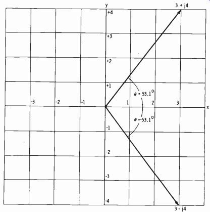
Fig. 2-10. Two vectors in rectangular form.
Table 2-5. Vector Rotation Due to j Operator
3 + j4
-3+j2
0+j6
The quantities may also be multiplied or divided, but it is more convenient to change from rectangular to polar form first (Fig. 2-10) . The polar form of 3 + j4 is 5 I°. The magnitude (5) is simply the vector addition of 3 + j4, or the hypotenuse of the right triangle whose other two sides are 3 and 4. The hypotenuse is equal to the square root of the sum of the squares of the other two sides.
The rectangular form can be converted to the polar form by use of the following trigonometric relationships:
sin 0 =
opposite side hypotenuse cos 0 adjacent side hypotenuse tan 6 = opposite side adjacent side The angle of the polar form may be determined first, even before the magnitude. Note that (in this example) the ratio of the opposite and adjacent sides of the right triangle containing the angle theta is already known to be 4/3, or 1.33. Then the angle whose tangent is 1.33 (from trigonometric tables) is approximately 53°.
If the rectangular form is 3- j4, the polar form is 5 /-53°.
Numbers in polar form may be multiplied conveniently. The numbers representing the magnitudes of the vectors in polar form are multiplied, and their corresponding angles are added algebraically. example:
(5 Z13°) (5 /-53°) =25 L°
Vectors in polar form may also be divided conveniently. To do this, di vide the vector magnitude in the numerator by the vector magnitude in the denominator; then algebraically subtract the angle in the denominator from the angle in the numerator. For example:
10 /+20°=2 /+30° 5
Polar form can be converted to rectangular form with the following relationship:
A /)=A cos 0+jA sin 0
For example, convert 5 / +53° to rectangular form. From trigonometric tables, cos 53° is 0.6, and sin 53° is 0.8. Then:
5 /+53°=5(0.6)+j5(0.8)
=3+j4
If angle 0 is negative, the relationship becomes:
A /-0=A cos O-jA sin 0
The resultant rectangular form of 5 /-53° is therefore 3- j4.
2-10. THE DECIBEL AND VOLUME UNIT
Understanding the terminology and correct usage of signal generators, meters, and measuring devices used in broadcasting is vitally important in testing and maintenance procedures. Therefore, this entire section is de voted to the units of measurement and their application.
When sound is increased in magnitude, the loudness is said to increase; the impression to the brain is roughly proportional to the logarithm of the ratio of the acoustical powers of the two sound levels. Loudness is a complex function dependent on many variables and is covered more fully in Section 11.
For example, suppose that a speaker driven with 1 watt has its driving power increased to 2 watts. It is meaningless to say that the power was increased by 1 watt unless it is also stated that the original power was 1 watt.
What is important is that the power was doubled. The ear interprets this as a certain change in loudness; but the same degree of change is perceived with an increase of only 1/2 watt if the original power was 1/2 watt, or with an increase of 2 watts if the original power was 2 watts.
The common logarithm of the ratio of two powers is an expression of their relationship in bels:
bels = log 10 P1 where, P1 is the reference power, P2 is the power being compared to P1.
The bel is too large a unit for practical use in radio work, so a unit equal to one-tenth of a bel, the decibel (dB) , is commonly used. Therefore the difference in level between P1 watts and P2 watts is given by:
dB = 101ogio (1.12) P1
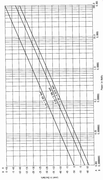
Fig. 2-11. Relationship of decibels and power level for three reference levels.
To avoid cumbersome computations, tables and graphs are normally used (see Table A-3 in Appendix A for the conversion of ratios to decibels).
Note that a power ratio of 2/ 1 is 3.01 dB; this is normally stated as 3 dB.
Zero dB (0 dB) may designate any convenient reference level. Although it is normally based on the ratio between two powers, the decibel can also be used to indicate absolute power, provided the reference level (zero level) is specified. In the past, so-called standard reference levels have been variously specified as 1, 6, 10, 12.5, and 50 milliwatts (mW) . The 1 mW reference level is most widely used today, but the practicing engineer will occasionally find 6 and 12.5 mW referred to as 0 dB. The term dBm is used to indicate that zero level is 1 mW. Note that power levels expressed in decibels are independent of impedance values. Fig. 2-11 shows a graph of decibels versus power for three reference levels.
Note from Fig. 2-11 that:
1. To convert from 1 mW reference to 6 mW, add-7.78 dB.
2. To convert from 1 mW reference to 12.5 mW add -10.97 dB.
3. To convert from 6 mW reference to 1 mW add +7.78 dB.
4. To convert from 12.5 mW reference to 1 mW add +10.97 dB.
With any reference level, a plus sign indicates so many "decibels up"; a minus sign indicates so many "decibels down." The statement of a power ratio in decibels is independent of reference level or impedance. The statement of absolute power in decibels is meaningless unless the reference level is stated.
When decibels are related to voltage or current, the value of impedance must be taken into account, since the voltage across or the current through an impedance depends on the impedance as well as the power level:
E = VWR where, E is the voltage across the impedance, W is the power in watts, R. is the impedance (purely resistive) in ohms.
Power is proportional to the square of the voltage or the current. When a number is squared, the logarithm of that number is doubled; therefore, when decibels are used to express voltage ratios, the following relation applies:
dB = 20 logo CE2) El
For current ratios, the relation is:
dB = 20 logo (I2)
\I,J
Table A-3 (Appendix A) lists decibels relative to voltage or current ratios as well as power ratios. Note that for a given ratio of power, the number of decibels is one-half the value for the same ratio of voltage or current.
The vtvm is a convenient tool that is often used in gain or loss measurements. Fig. 2-12 shows the dBm-to-volts relationship for the impedances given.
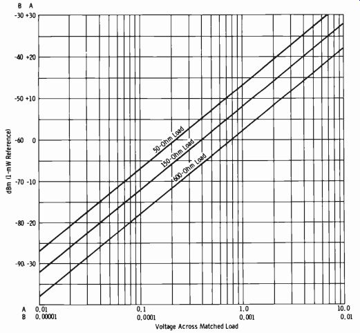
Fig. 2-12. Relationship of dBm and load voltage.
Volume Units and VU Meters
The VU meter is a standardized instrument intended for the monitoring of radio-program content. Since the power in program signals is constantly fluctuating, the meter reading must be standardized as to whether it is peak, rms, or average, and the meter movement must have specified ballistic characteristics, such as speed of response and damping.
The standardized VU meter employs a full-wave dry-disc rectifier. Its dynamic characteristics are such that if a sinusoidal voltage in the frequency range concerned and of such amplitude as to give reference deflection (under steady-state conditions) is suddenly applied, the pointer will reach 99 percent of reference in 0.3 second ( within 10 percent) . The pointer will then overshoot reference deflection by a minimum of 1 percent and a maximum of 1.5 percent.
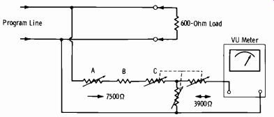
Fig. 2-13. External circuit of standard VU meter.
Fig. 2-13 illustrates the conventional external circuitry involved with the use of the standard VU meter for monitoring transmission levels. In practice, the signal level is such that the range of the meter must be extended. The impedance of the meter itself varies with the voltage across the meter terminals and, therefore, must be isolated by a resistance net work. The ballistic characteristics described are dependent on the meter load impedance, which must be 3900 ohms. The decibel reading of the calibrated, variable meter multiplier (C) plus the scale reading of the meter yield a measurement of the transmitted level. The complete network contains the following components:
A. Zero adjuster, approximately 800 to 1000 ohms.
B. Fixed resistor, approximately 3200 ohms, selected so that with A at mid-position, A + B = 3600 ohms C. Meter multiplier, "T" attenuator, 3900 ohms input and output.
The meter input impedance, as seen by the program line, is 7500 ohms, except when a 1-mW position is provided. This is for a test position only and is not used in program monitoring.
The volume unit implies a complex wave, a waveform with a higher peak-to-rms ratio than a sine wave. When the VU meter is used to measure steady, single-frequency sine-wave signals, the reading should be referred to as so many dBm. Volume units should never be used to indicate the level of a sine-wave signal.
The volume unit has as its reference a steady-state condition, however.
This reference is 1 mW of sine-wave power at 1 kHz through a resistance of 600 ohms. When the instrument (having an internal impedance of approximately 3600 ohms) and an external calibration potentiometer are connected across such a circuit, the indication should be 0 VU. However, when the meter is bridged across a 600-ohm program circuit as shown in Fig. 2-13 (total bridging impedance of 7500 ohms) , the maximum sensitivity of the meter is +4 dBm for 0 VU. Most program lines are fed with a +8 dBm level. In this case, the external multiplier is set to +8, and the meter indicates 0 VU at +8 dBm.
The VU meter is, by definition, properly calibrated only when connected across 600 ohms. When it is connected across any impedance other than 600 ohms, the reading must be corrected by adding 10 log10 (600/Z), where Z is the actual impedance in ohms. The EIA and FCC specifications for noise and distortion measurement require that a meter with standard VU characteristics be used. In this case, the meter on the measuring equipment reads an actual 1 mW of sinewave power in 600 ohms for zero reference.
Always remember the basic differences in terminology between program and test signals, which may be summarized as follows: Reference volume is that strength of program signals that causes 0 VU (or 100 percent) deflection under the conditions described. This definition is arbitrary be cause the complex nature of the waveform makes a definition in fundamental terms impossible. Reference level is that steady-state condition in which there is 1 mW of a 1000-Hz sine wave in a 600-ohm impedance across which the meter indicates 0 reference level. This should be termed 0 dBm. However, when the meter is connected per standard practice ac cording to Fig. 2-13, the maximum sensitivity is +4 dBm for 0 VU deflection. The actual level is the setting of the multiplier in decibels plus the meter reading. Some multiplier arrangements allow a 1-mW position for test purposes only; this position taps down on the attenuator for a lower multiplier resistance.
Decibels In Practice
The first consideration is feeding the output of the sine-wave signal generator to the input of the system or device being tested. (Actual techniques are covered in Sections 13 and 14. Only the proper reading of decibels is of concern here.) Fig. 2-14 shows a typical arrangement. The generator dBm meter is always loaded by the constant impedance of the output transformer. The actual output is the reading of the meter minus the setting of the calibrated attenuator. For example, to feed a microphone preamplifier, the generator gain might be adjusted to give a meter reading of +15 dBm and the attenuator set to 65 dB. The actual output is then 15- 65 =-50 dBm, a typical value for the input circuit of a micro phone preamplifier.
The generator output-transformer secondary is then adjusted (usually by means of a switch connected to transformer taps) to match the load, which is the input of the preamplifier. This is normally 600, 150, or 50 ohms. The actual dBm input to the device is independent of the value of the load. Zero dBm sets the reference level at 1 mW in any load.
The voltage developed across the load and the current through the load are dependent on the value of the load in ohms. For example, 0 dBm (1 mW) results in 0.774 volt across 600 ohms, 0.387 volt across 150 ohms, and 0.224 volt across 50 ohms (Fig. 2-12) .
Provided the generator output is matched to the load impedance, no con version in meter reading (in dBm) is necessary when feeding the device or system, regardless of the input impedance. This is simply a practical application of Ohm's law, but it has resulted in some confusion in practice.
The explanation of why the power remains the same regardless of impedance should be reviewed, as follows.
When the impedance is reduced from 600 to 150 ohms, the ratio is 4/1.
Since the turns ratio of the output transformer is the square root of the impedance ratio:
Tranformer
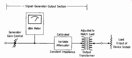
Fig. 2-14. Connection of signal generator to system being tested.
Turns ratio = \/600/ 150 = = 2 to 1
Since the voltage developed is in direct proportion to the turns ratio, just one-half the voltage is developed across 150 ohms as for 600 ohms at any reference level. However, calculation shows that the same power exists in the load for either case. Therefore the level indicated on the generator dBm meter (minus the attenuator setting) is the actual level at the system input, provided the impedances are matched.
When the load does not match the output impedance of the generator, it is convenient to measure the voltage gain and then convert to decibels.
The generator is adjusted to the closest match available, and the following calculation performed:
RL ET =EocRL+Ro where,
EL is the voltage across the external load, Eoc is the open-circuit voltage (twice the voltage that would appear across a load equal to Ro), RL is the external resistance load, Ro is the output impedance of the generator.
For example, assume that the external load is 250 ohms, the generator output impedance is set at 150 ohms, and the generator output is-10 dBm.
From Fig. 2-12 the voltage across a 150-ohm load would be 0.125 volt, so Eoc in this example is 0.25. Substituting in the formula gives:
250 Et. = 0.25 250 + 150 = 0.25 250 400 = 0.156 volt
Note from Fig. 2-11 that-10 dBm represents a power of 0.1 mW. The power (E2/R) in the 250 ohm load is:
0.1562
0.0243
0.097 mW
250 250
This is less than 0.5 dBm from the-10 dBm reference of 0.1 mW, an error that normally may be disregarded. Unless the mismatch is 2/1 or greater, any correction factor usually can be ignored except for the most precise measurements.
As mentioned previously, noise and distortion measurements are made with a meter that has standard VU characteristics to meet EIA and FCC specifications. This VU meter is properly calibrated only when reading across 600 ohms. For example, assume it is necessary to measure the gain of an amplifier with 150 ohms input and output. Further assume that the gain of the amplifier is 40 dB. If the input is to be-20 dBm, the output should be +20 dBm. As described, the generator should feed-20 dBm into the amplifier, and no conversion factor is involved. However, the output must be measured with a meter calibrated in dBm for 600 ohms. It has been noted that the impedance ratio between 600 ohms and 150 ohms is 4/1, which, for a given power, corresponds to a voltage ratio of 2/1.
A 2/1 voltage ratio is equal to 6 dB (Fig. 2-12 or Table A-3) . Therefore, the meter reading is 6 dB low across 150 ohms, and the correction factor is +6 dB. Then the meter at the output of the amplifier should read 20- 6, or +14 dBm. The actual output is then 14 + 6 = 20 dBm. Fig. 2-15 gives the correction factor for impedances from 10 ohms to 10,000 ohms, for the reference 0 dBm = 1 mW in 600 ohms.
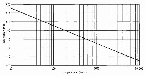
Fig. 2-15. Correction factor for VU meter across various impedances.
Note that with the usual broadcast-type signal generator and measuring equipment no correction factor (in dBm) is involved at the system input.
But if the measurement is made across other than 600 ohms at the output, the proper correction factor must be applied to the reading.
There are many applications in practice in which the standard VU meter is used across impedances other than 600 ohms. It is important to understand the proper interpretation for maintenance and level setting. For example, it may be desirable to monitor all inputs to a crossbar switcher where all the inputs are 150 ohms. Assume the proper level at this point is +10 dBm. If the standard minimum insertion loss multiplier is used, the level across 600 ohms would be +4 dBm for 0 VU deflection. However, the correction factor for 150 ohms is +6 dB. Therefore, 0 VU deflection now indicates 0 dBm +4 dB +6 dB, or +10 dBm in 150 ohms.
Now further assume that an external test decibel meter which does not employ the program-line bridging network is used, and the reference level of 1 mW in 600 ohms is stated on the scale of the meter. In this case, the 150-ohm crossbar input level should indicate +4 dBm (0 dBm with the external multiplier set on +4) . Then with the +6-dB correction factor, the actual level is +10 dBm.
The preceding information is important to the installation engineer and to the maintenance department. Once the VU meters are installed in a system, the operating engineer is not interested in absolute levels; he only needs to see that the program level is maintained at the zero reference level on peaks.
Always bear in mind that when a VU meter peaks at 0 VU or 100 percent on program material, actual instantaneous peaks will occur at well over 1 mW in 600 ohms. This peak factor of the average program wave is generally taken to be 10 dB over the peak-to-rms value of a sine wave.
For this reason, a unit or system is sometimes tested and measured with a sine-wave power of 10 dB above the program operating reference. The Bell Telephone test board commonly feeds tones at 10 dB over the pro gram operating level when measurements for distortion and cross talk are being made. This is important to the operator who may be monitoring the incoming network line for purposes of setting level on network circuits.
When there is any doubt, the local test board concerned should be contacted to ascertain the level being transmitted.
Microphone Output in Decibels
A microphone output may be expressed in terms of either voltage or power. Since the output is obviously dependent on the magnitude of excitation, the reference is normally made to either 1 or 10 dynes per square centimeter. (A level of 0.0002 dyne/cm2 is considered to be the threshold of audibility.) All microphone output ratings are expressed at a single stated frequency.
When the output rating is given in terms of voltage, the reference is 1 volt (open circuit) , usually at 1 dyne per square centimeter. The expression is abbreviated dBV, which indicates decibels with a reference of 1 volt as 0 dB. Thus if a microphone specification sheet states the output as -60 dBV, this indicates that an open-circuit voltage of 60 dB below 1 volt is generated with a sound pressure of 1 dyne/cm^2. When the microphone is connected to a matched load, the voltage is decreased to one-half the open circuit voltage, or 6 dB less. The effective output is then -66 dBV. Note in Table A-3 that -60 dB indicates 0.001 of the reference voltage, or 1 millivolt (open circuit) . An additional 6 dB cuts this value in half, giving an effective 0.5-mV signal.
Most broadcast-type microphones are rated in terms of power output (dBm) at a stated sound pressure. Typical ratings are from -50 to -65 dBm at a sound pressure of 10 dynes/cm^2. Note that 10 dynes/cm^2 is 50,000 times the pressure at the threshold of hearing, 0.0002 dynes/cm^2.
A voltage ratio of 10,000/1 is 80 dB. The ratio of 50,000 to 10,00 is 5, which gives an additional 14 dB and a final level of 94 dB above threshold level. This is in the upper region of the average program sound pressure encountered in practice. (See Fig. 2-16, which is a graph of sound level ranges in dynes/cm^2 relative to decibels, where 0.0002 dyne/cm^2 is 0 dB at 1000 Hz.) The EIA (formerly RETMA) microphone system rating is also a power rating, but it is a ratio in decibels, relative to 1 mW and 0.0002 dyne/cm^2, of the power available from the microphone to the square of the undisturbed sound field pressure in a plane progressive wave at the microphone position. (This simply specifies the axis of the microphone relative to the sound front.)
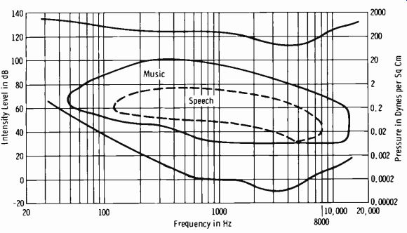
Fig. 2-16. Sound-level ranges.
The EIA system rating is given by:
GM = 120 log1 P
- 10 log1) RMR I- 50 dB where,
GM is the microphone system rating (sensitivity) in dBm, E is the open-circuit voltage generated by the microphone, P is the sound pressure in dynes per square cm, RMR is the microphone rating impedance.
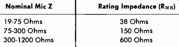
Table 2-6. Microphone Impedance Ratings
Nominal Mic Z Rating Impedance (R NI 10
19-75 Ohms 75-300 Ohms 300-1200 Ohms 38 Ohms 150 Ohms 600 Ohms
Microphone rating impedances (RMR) for broadcast-type units are given in Table 2-6.
Note that you can convert readily from the EIA microphone system rating to the effective output rating in dBm. It is only necessary to consider the difference in acoustical pressure between 0.0002 dyne/cm^2 and 1 or 10 dynes/cm^2. The ratio of 1 to 0.0002 is 5000/1, or 74 dB. The ratio of 10 to 0.0002 is 50,000/1, or 94 dB, as discussed previously. Thus to convert from a GM rating to effective output, for 1 dyne/cm^2 add 74 dB and for 10 dynes/cm^2 add 94 dB. For example, if a certain microphone has a GM rating of -150 dBm, the effective output level at 1 dyne/cm^2 is-150 + 74 = -76 dBm. At 10 dynes/cm^2, the effective output level is -150 + 94 =- 56 dBm.
A natural question that may occur at this point is why the voltage ratio is used in expressing pressure ratios in terms of decibels and then also is used in adding to a power level in dBm. Actually, when a microphone is connected to an unloaded input transformer, its output cannot be expressed in power since no appreciable power is delivered. The effective output level of the microphone is simply that level which, when added to the amplifier power gain in dB, gives the correct output level from the amplifier in dBm.
The effective output level of a microphone connected to a matching impedance is given by:
z Po = 1000 Rnrt where, Po is the output level in milliwatts, EG is the open-circuit output in volts, RM is the nominal microphone impedance.
The power in milliwatts can then be converted into dBm.
Radio-Frequency Applications of Decibels
The field strength of a radio-frequency wave is conveniently stated in terms of dBu, where 0 dBu = 1 microvolt per meter (µV / m) . Note that this simply involves a voltage ratio. Power is conveniently stated in terms of dBk, where 0 dBk = 1 kW. This simply involves a power ratio.
There are three primary advantages of using decibels to express field strength (volts) and power ( watts) :
1. Antenna power gain in dB may be added directly to transmitter power level in dBk.
2. Antenna field gain in dB may be added to received field strength in dBu. That is, an increase of 1 dB at the transmitter antenna results in an increase of 1 dB in received field strength.
3. Transmission-line losses in dB may be subtracted directly from transmitter power output in dB above or below 1 kW.
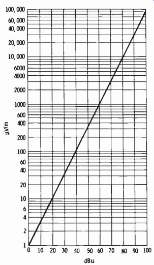
Fig. 2-17. Graph relating dBu to microvolts per meter.
For convenience, Fig. 2-17 is a graph relating dBu to actual microvolts per meter. Fig. 2-18 is a graph relating dBk to actual watts of power. Fig. 2-19 relates percent efficiency to decibels of attenuation and is particularly useful for handling transmission-line characteristics in the calculation of effective radiated power.
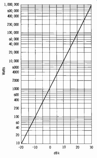
Fig. 2-18. Graph relating dBk to power in watts.
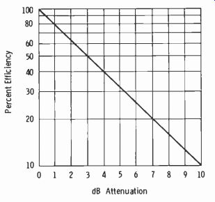
Fig. 2-19. Graph relating percent efficiency and dB attenuation.
To apply decibels to some familiar figures in broadcasting, consider the 3.16 mV/m required to be delivered by an fm station over the principal city to be served. This can be expressed as 70 dBu. The outer limit of service for an fm transmitter is 50 µV/m, or 34 dBu. Note from the graph in Fig. 2-18 that since 0 dBk = 1 kW (1000 watts), 0.1 kW (100 watts) =-10 dBk and 10 kW (10,000 watts) = +10 dBk.
Effective radiated power (erp) is a measure of the actual signal strength radiated by the station. It depends on the transmitter power output, trans- mission-line attenuation, and antenna gain. For example, assume that the transmitter power output is 10 kW, the transmission-line efficiency (for type, frequency, and length of line required) is 79 percent, and the antenna power gain is 3.2. Note that if the conventional computation of erp is made, it is necessary to take 79 percent of 10,000 and then multiply by 3.2 to obtain the erp (25,280 watts) . However, the computation can be carried out as follows:
10 kW = +10 dBk 79 percent efficiency = 1 dB attenuation (Fig. 2-19) Power gain of 3.2 = 5 dB (Table A-3)
Then:
+10- 1 + 5 = +14 dBk
Note the simple addition and subtraction for the erp in terms of dBk.
This is obviously still more simplified when the transmission-line attenuation and the antenna gain are specified in decibels, as some manufacturers list them.
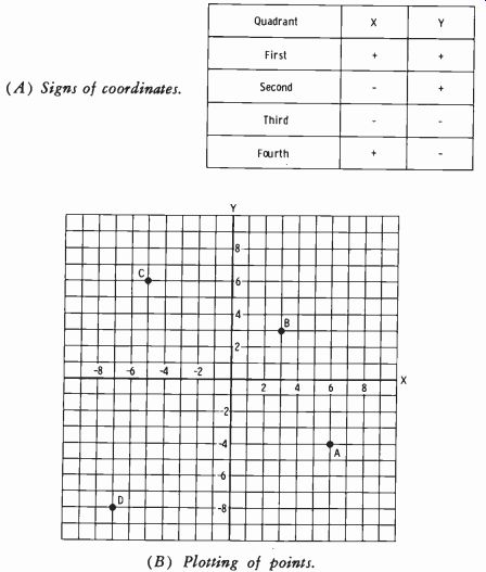
Fig. 2-20. Rectangular coordinates. (A) Signs of coordinates. (B) Plotting of
points.
2-11. THE CURVE AND THE GRAPH
Graphs (such as those of Figs. 2-17, 2-18, and 2-19) are widely used in electronics for a pictorial presentation of algebraic and/or geometric functions. On a graph, adjacent points may be joined by straight lines, or a sufficient number of points may be plotted to permit drawing a smooth curve.
A common example of the latter is a graph of the amplitude-versus-frequency response of an amplifier or complete system.
Graph Paper
Graph paper is available in a wide variety of forms, including rectangular-coordinate, logarithmic, polar-coordinate, and many special-purpose types. Fig. 2-20 is a basic example of the rectangular coordinate system.
Four points are plotted in Fig. 2-20B. For point A, x = 6 and y =-4; for B, x = 3 and y = 3; for C, x =-5 and y = 6; for D, x =-7 and y =-8.
Conversely, if point A is known, the x and y components of A may be found by extending lines from A to the corresponding points on the x and y axes.
When a plot must be made covering a wide range of values, either log-log scales or semilog scales are employed. "Log-log" means that both the x and y axes are marked with logarithmic scales. On semilog paper, one scale is logarithmic and the other is linear. For example, the usual scale used for plotting amplitude-versus-frequency response is logarithmic along the x axis and linear along the y axis. (For an example, refer to Fig. 5-5 in Section 5.) An example of polar-coordinate paper is illustrated in Fig. 2-21. Note that the scale is marked in degrees both clockwise and counterclockwise.
For directional-antenna patterns, the reference line is north (0°), and the angles are measured clockwise.
Smith Charts
Interpretation of some measurements made on transmission lines and waveguides may be made on a Smith chart. This form of transmission-line chart is a polar plot, consisting of a system of impedance coordinates, super imposed upon which is another system of lines representing loci of constant standing-wave ratio and constant distance along the line. The chart may be used for the interpretation of the measured values of vswr and the location of the voltage minima in terms of equivalent input impedance (or admittance) circuits, or in terms of reflection coefficients. It is also useful for determining the effect of a discontinuity or a change in characteristic impedance, and for solving impedance-matching problems.
Point X at the center of the chart (Fig. 2-22) is the origin for a polar plot of the reflection coefficient. The angle is indicated on the circular scale around the rim, and the magnitude is indicated by the radial distance measured outward from the center on a scale graduated linearly from 0 to 1.
Circular arcs, such as A, extending from point Y to the outer rim are the loci of all reflection coefficients that correspond to normalized impedances having equal reactive parts; for arc A, the impedances have a reactance of 1.0. Circles such as B represent reflection coefficients corresponding to normalized impedances having equal resistive parts; for circle B this resistance is 0.8.
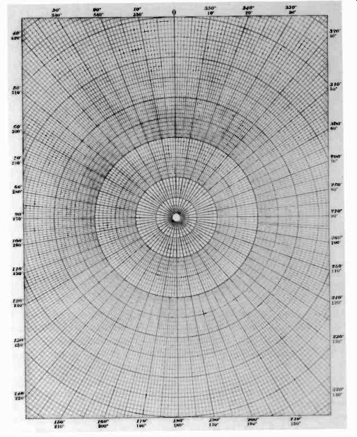
Fig. 2-21. Example of polar-coordinate paper.
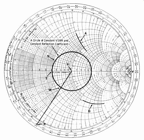
Fig. 2-22. Smith chart.
In traversing a standing-wave circle (S) with a standing-wave ratio of 2.0, the resistance axis is crossed at two points, one giving a very high resistance and the other a very low resistance. These correspond to the voltage maxima and minima, respectively, observed on a standing-wave detector.
On the basis of this, the Smith chart can be used in connection with the standing-wave detector to determine unknown load impedances. For ex- ample, a standing-wave ratio of 2.0 (circle S) is observed, and the first voltage minimum is 0.08 wavelength (R) from the load. Starting at point T, which corresponds to the voltage minimum at a standing-wave ratio of 2.0, travel along this circle (S) of constant standing-wave ratio toward the load to the point where the line drawn between points R and X intersects circle S. At this point of intersection (W) read the coordinates of the load impedance, which in this example are 0.62 - j0.38. Multiplying these numbers by the characteristic impedance of the standing-wave detector gives the actual impedance of the terminating load.
EXERCISES
Q2-1. Add: 4, 7,-10, 8,-6, 9
Q2-2. Add: 21, 5,-30, 2,-16
Q2-3. Subtract-16 from 5.
Q2-4. Multiply 4/5 by 3.
Q2-5. Divide 9/32 by 3.
Q2-6. Solve: 1/7 + 1/3 + ½
Q2-7. Solve: 1/4- 1/6
Q2-8. (2/3)(1/5) = ?
Q2-9. (3/4)(6/10) _ ?
Q2-10. Divide 2/3 by 3/5.
Q2-11.
40 (5)33) + (45)(4)-5 = ?
Q2-12.
The no-load voltage output of a power supply is 48 volts, and the full-load voltage output is 47.5 volts. What is the percentage regulation?
Q2-13. 10° = ? 4° = ? 2° = ?
Q2-14. (5--4)(53)(52)(5-9) = ?
Q2-15. (A) (45)3 = ? (B)(4-5)-3= ? (C) (4-5)3 = ? (D) (42)-6 = ?
Q2-16. (3/4)2 = ?
Q2-17. x/69,573 = ?
Q2-18. 4(10)3(5)(10-12)(2)(106) 5(107)(4)(1016)
Q2-19. (A) Log 1000 = ? (B) Log 100 = ? (C) Log 10 = ? (D) Log 1 = ? (E) Log 0.0001 = ?
Q2-20. Log10 54.65 = ?
Q2-21. Multiply 1.24 by 246 using logarithms.
Q2-22. Divide 961 by 224 using logarithms.
Q2-23. 6385 = ? Use logarithms.
Q2-24. If X = AB B=? A=?
Q2-25. In Fig. 2-8, assume A = 10 / 30° and B = 5 / 60°. What are the magnitude (R) and angle (r) of the resultant vector?
Q2-26. Convert 20 / 30° to rectangular form.
Q2-27. Convert 30 + j50 to polar form.
Q2-28. One dBm = ?
Q2-29. If the input to a transmission line is 150 watts and you measure 100 watts at the output end of the line, what is the loss in decibels?
Q2-30. What is the power gain of an amplifier rated at 40 dB gain?