10.1 OBJECTIVES AND TERMINOLOGY OF STATISTICS
Descriptive statistics attempts to summarize a mass of data in a few meaningful numbers. Omega University may have 5000 students receiving 20,000 individual grades, but we can speak of the average grade as being 2.72, and the increase in average grade as averaging 0.02 per year over the past 10 years, and the number of E grades as being 6% of the total.
Inferential Statistics attempts to make generalizations about a large group by gathering and analyzing data from a relatively small sample of that group. Thus, although there is no central data bank containing the height measurements of every 21-year-old female in the United States, and we do not have the resources to gather such data, we can nevertheless state with almost complete certainty what the average value is, what percentage is below 62 in., or above 66 in., or whatever other number we choose. This is possible because we have data from a small but carefully chosen sample of this unmanageably large group. Most of this section is devoted to techniques for drawing inferences about large batches of electronic components from analysis of smaller samples.
Population is the name given to the entire group under concern. Often it is an indefinite large number, as in the case of components under continuous production. We denote the number of items in the population with the letter N.
Sample is the part of the population for which data are gathered. A random sample (the only useful kind) is one in which each member of the population is equally likely to be selected for the sample. Obtaining a random sample is often more difficult than it would seem. A political survey would be nonrandom or biased if it were taken in a single city or region or if it were taken by phone (certain types of people tend to have unlisted numbers) or by mail (certain types tend not to respond) or in person (certain types don't answer the door for strangers). In industry, random sampling generally requires that components be selected from different boxes, at different times of the day, from the beginning, middle, and end of a production run. One of our major objectives will be to determine the minimum sample size required to adequately represent the population. We denote sample size by n.
Score is the measured value of a parameter, be it ohms, volts, microfarads, or whatever.
We term them Xt, X2,, Xn, and, where two samples are involved, Yx,Y2,...,Yn.
Mean is the statistical term for average. It is calculated by summing all the scores and dividing by the number of such scores. We denote population mean by fi and sample mean by X and Y.
(10-1)
(10-2)
Level of Confidence is our degree of certainty about an inference that is drawn from a sample. Say that we wish to know whether Ajax or Zeus brand resistors have a tighter tolerance. We select samples of 10 resistors from each company and find that the Ajax sample has an average deviation of 4%, whereas the Zeus sample averages 5% deviation. The Zeus representative complains that it was just bad luck that some of the worst of his company's resistors were selected and compared to some of the best from Ajax. In other words, the sample was not typical of what would be expected if we drew several such samples. So we pull 10 times the sample size-a total of 100 from each company-and find Ajax averaging 4.6% and Zeus averaging 4.3% deviation. Now the Ajax rep complains that the luck of the draw was against him. But it is harder to argue bad luck in such a large sample. If a man loses at poker one night, he may have had bad luck, but if he loses nine out of 10 nights, we become quite sure that he is simply a poor player.
We can calculate and express our level of confidence precisely as a percentage.
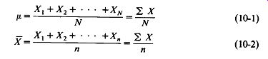
A confidence level of 95% means that if we repeated our sampling test 100 times on two populations which were in fact identical, five of these tests would judge the populations to be different, just because the samples drawn would be atypical. A 95% level of confidence is sometimes spoken of as 0.05 level of significance. Figure 10-1 illustrates these concepts.
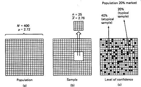
FIGURE 10-1 (a) Illustration of a population of 400 and its mean score /i.
(b) Illustration of a sample of 25 from the population of 400, and the mean
score of the sample X. (c) Illustration of the possibility of drawing a sample
that Is not typical of the population.
Normal Distribution: Quantities of measured data can be summarized by constructing a bar graph (called a histogram) as shown in Fig. 10-2(a), which purports to represent the distribution of capacitance values of a sample of 24 nominal 1.0-uF capacitors. Class intervals of 0.1 uF are used. There are, for example, 5 capacitors in the interval between 1.1 and 1.2 uF. If a very large sample were taken, we might wish to use smaller intervals to obtain a more accurate picture of the distribution, and a histogram like the one in Fig. 10-2(b) might be obtained.
If the sample size is made indefinitely large and the class intervals are made indefinitely small, we obtain a smooth frequency-distribution curve, as shown in Fig. 10-2(c). In a remarkable number of real-life applications, the shape of this distribution curve approaches a mathematical ideal called the normal curve, or somewhat loosely, the bell curve. Grade-point averages, IQ test scores, height of army inductees, values of resistors produced by a given machine, and number of defective parts in a day’s production run, to take a few examples, all tend to be normally distributed. Most of the techniques presented in this section assume that the population in question is reasonably close to a normal distribution.
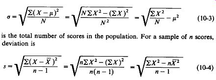
Standard Deviation is a measure of dispersion or central tendency which is essential in dealing with the normal curve. Data that are widely scattered above and below the mean have a large standard deviation. Closely grouped data have a small
FIGURE 10-2 Histograms showing the distributions of scores: (a) small sample
size; (b) large sample size; (c) theoretical normal distribution, showing
the fraction of scores lying 1, 2, 3, and beyond 3 standard deviations from
the mean.
The total area adds to 1.000. standard deviation. Standard deviation for an entire population is calculated as:
(10-3)
... where N is the total number of scores in the population. For a sample of n scores, standard deviation is: (10-4)
The first forms given are the defining equations, but they may prove inconvenient for calculation since they require subtraction of the mean and squaring for each score. The second forms given are for calculation from raw score data, and the third forms are for calculation from raw scores once the mean has been obtained.
Areas under the Normal Curve: The total area under the normal curve is 1.000.
The number of scores included within ± 1 standard deviation is 0.6826 of the total.
The fraction lying within ±2 standard deviations is 0.9544, while 0.9972 of all scores fall within ±3 standard deviations. This is illustrated in Fig. 10-2(c). Table 10-1 gives "tail areas," that is, the proportion of scores lying beyond the given number of standard deviations from the mean in one direction.
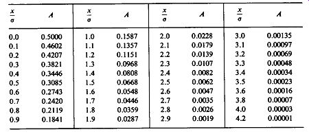
TABLE 10-1 Tail areas under the normal curve, one side. Where deviation
from the mean X - X - x, x/o - standard deviations above or below the mean.
A - area from x/o to infinity, one side.
10.2 DESIGN OF STATISTICAL EXPERIMENTS
Now that you have the basic terminology in hand, you may feel ready to set up a statistical experiment and analyze the results. However, it is often said that a little knowledge is a dangerous thing, and you should be aware that the information contained in this section is only enough to make you dangerous. Where matters of importance are involved it is recommended that you consult a full-fledged statistics text or, better still, a full-fledged statistician. The primary benefit of this section should be to make you aware of the possibilities of statistical analysis and to allow you to converse intelligently with those who can handle the analysis properly. This section consists primarily of a list of thou-shalt-nots in designing your experiment.
Randomize Your Data: This almost always requires that a special sample be drawn for the experiment, which involves staying late to catch the second-shift foreman, and digging down to the bottom rear of a warehouse stack for a sealed carton that has no other reason for being opened. The boss may object and tell you to pull your samples all from one already-available box, but the results cannot then be supported. Each member of the population must have an equal chance to be selected for the sample, so discriminating against hard-to-obtain data cannot be tolerated.
Every dog has its day, and every problem-ridden production line will, by luck, eventually produce a crate of gems. In a competitive economy the temptation to zero in on such good fortune and produce a "statistical study" is almost irresistible.
Such tactics are pernicious, but they are perpetrated every day on the gullible.
Non-normal distributions can destroy the validity of sampling tests that assume a normal distribution. The values of the resistors in a particular shipment, for example, may be normally distributed except that all values above and below 2.5 standard deviations from the mean have been eliminated from the population by the vendor [Fig. 10-3(a)]. Bimodal distributions [Fig. 10-3(b)] may be ob served where two machines are used to produce components, which are then batched together. Drastically skewed distributions [Fig. 10-3(c)] are occasionally encountered.
A histogram plot with 8 to 20 class intervals and a sample size of 30 to 100 is probably the most practical device for verifying that a distribution is essentially normal. Mathematical "goodness of fit" tests do exist, but they are quite complex.
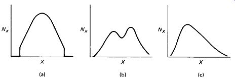
FIGURE 10-3 Non-normal distributions: (a) selective elimination; (b) bimodal;
(c) skewed.
Hawthorne Effect: Several decades ago industrial engineers at a major tele phone-equipment assembly plant decided to investigate the effect of lighting on worker productivity. They found that when lighting levels were increased production went up-and that when lighting levels were decreased production went up-and that when they simply stated their intent to change the lighting, production went up. Of course, the workers were reacting not to the lighting but to the fact that they were being studied. It may have made them feel " under the gun" or it may have made them feel especially important, either feeling tending to increase production.
The serendipitous lesson of the Hawthorne study should not be overlooked, but where a statistical study of some Variable other than worker attitude is being undertaken, care must be taken to see that worker attitude does not bias the results.
One tactic is to hide from the workers the fact that they or their products are under study, at least until after the samples are obtained. Where this is not possible, it is advisable to form two groups of workers for comparison, and tell both that they are part of a study. Under no circumstances should the performance of people who knew they were under study be compared with the performance of people working under the " same old grind. "
Statistical Errors: In sampling statistics the possibility always exists that we will accept a bad batch of components or reject a good batch just because we have been unfortunate enough to draw an atypical sample. Large sample sizes minimize this possibility, but they do not eliminate it.
10.3 DIFFERENCE BETWEEN MEANS
For our first statistical study we will analyze a sample to determine whether there is a discernible difference between the means of two populations. Consider the case of two competing brands of capacitors. We wish to determine which brand has the higher breakdown voltage. We cannot be confident that samples of one or two of each brand will be representative of the populations, but the test is destructive and fairly time consuming so we don't want to use a larger sample than necessary. How can we determine when we have a large enough sample to establish with a desired level of confidence that one brand is better than the other? We begin by randomly selecting five capacitors of each brand. We calculate the mean and standard deviation of each sample according to equations 10-2 and 10-4. We then calculate the value of a parameter known as t:
(10-5)
... where n is the number of items in each sample. We then consult Table 10-2 of / values to determine what, if any, significance can be attached to the difference in sample means X - Y. If the level of confidence thus established is unsatisfactory, we can draw five additional capacitors of each brand and repeat the calculations for X, Y, sx, sy, and t with n = 10. If the results are still unsatisfactory, we can proceed to n = 15, 20, 30, and 100 in an attempt to establish the desired level of confidence that one population mean really is greater than the other.
TABLE 10-2 Critical values of t.
Table 10-2 is quite abbreviated to suit the purposes of this introductory section. More complete tables of t, which may be found in any statistics text, will no doubt list degrees of freedom (df) in place of the sample size (n) column. The concept of degrees of freedom and how it relates to sample size is too involved to attempt an explanation at this time, but understand that the two are not equal.
EXAMPLE 10-1
Five brand X and five brand Y capacitors were randomly selected and destructively tested for breakdown voltage with the following results:
X (V) Y(V) 450 550 510 520 470 490 580 550 470 570
Can we state with confidence that one brand has a higher average breakdown voltage than the other?
Solution
----
Consulting Table 10-2, we find that t = 1.48 is sufficient to establish an 80% confidence that Y averages a higher breakdown voltage than X.
Statisticians consider 95% confidence to be acceptable for general applications, but require 99% confidence where the consequences of a wrong decision would be severe.
We would probably want to take an additional five samples of each brand and calculate t with 10 in an attempt to gain a higher level of confidence in our decision.
Note that the t test, as it is called, merely establishes a level of confidence that one population mean is greater than the other. It does not establish how much difference there is between fix and In Example 10-1, our best estimate of the population means is u_x = 496 V and u_y = 536 V, but we are by no means 80% confident that these are the true population means or that the true means differ by this amount.
If political and economic considerations were such that we would require demonstration of, for example, a 25-V difference in the means before we would consider switching from brand X to brand Y, we could simply subtract 25 V from each brand Y score in the sample before conducting the t test. The result would be our level of confidence that u_y exceeds u_x by at least 25 V.
10.4 DIFFERENCE IN DISPERSION
Sometimes we are interested not in the means of two populations, but in the narrowness of their distribution curve. In comparing two resistor-molding machines, a resistor manufacturer would choose the one that produced the smaller spread of values, since this machine would produce fewer out-of-tolerance resistors.
To establish whether a discernible difference in dispersion of two populations exists, equal samples are drawn from each population and the standard deviation of each sample is computed. The larger s is then divided by the smaller s, and the quotient is squared, producing a parameter called F. A table of critical values of F is then consulted to determine the significance of the difference in standard deviations (Table 10-3).

(10-6)
TABLE 10-3 Critical values of F.
EXAMPLE 10-2
Two machines were set up to produce 1000-ohm resistors.
A sample of 10 was drawn from each machine>s run with the following results:
1001 1011 959 1002 1027 995 973 991 1035 1017 965 984 1004 1064 989 976 1052 1018 967 972
Can we state with confidence that one machine produces a closer grouping of resistors than the other?
Solution
This value of F falls short of establishing a 90% confidence that population standard deviation ay really is smaller than ax, and we would again call for a larger sample. Table 10-3 and equation 10-6 reveal that samples of 200 will give 90% confidence in the existence of a difference when that difference i s only 13%. If this is considered trivial we would decline to take so large a sample and report essentially identical populations if a significant value of F could not be achieved with smaller samples.
10.5 CORRELATION
In many cases the parameter of interest cannot easily be measured directly, and we must seek to establish a correlation between the critical unmeasurable parameter and some other readily observable parameter. Such instances often arise when the critical parameter involves a destructive effect, such as insulation breakdown or fuse-element melting.
The author was once involved in the manufacture of a computer disc memory which was plagued by low-amplitude recording at certain of its 64 record heads.
Replacing a defective head was a very expensive procedure since the entire unit was sealed in an inert gas. It was alleged that potential low-amplitude heads could be spotted by measuring their impedances before the memory was sealed and replacing heads with unusually low impedances. In other words, it was alleged that there was a high correlation between record amplitude and head impedance.
The idea of correlation is illustrated very nicely by a scatter diagram, as in Fig. 10-4. If the correlation is obviously strong, the diagram itself will be the most ...
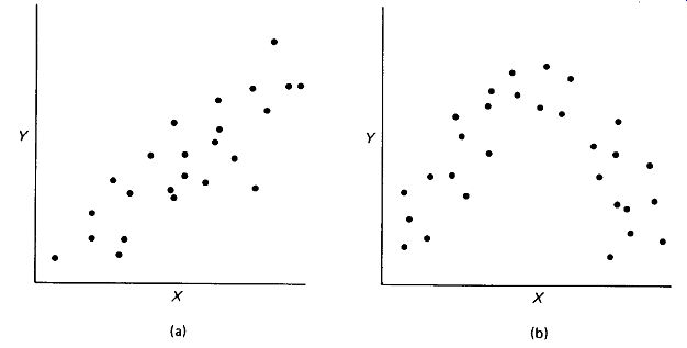
FIGURE 10-4 Strong linear correlation between X and Y is evidenced by the
scatter diagram (a). Nonlinear correlations (b) are not amenable to the tests
of Section 10.5.
... convincing tool, but if the correlation is not so obvious, or if the sample size must be kept as low as possible, we will want to calculate the numerical correlation coefficient r. Note that the r computation assumes a linear relation between X and Y, as in Fig. 10-4(a). A curvilinear relation, as in Fig. 10-4(b) cannot be handled by this technique. The correlation coefficient is calculated as:
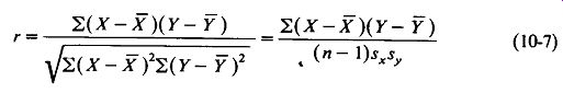
(10-7)
The second form of the equation is given to facilitate calculation where the standard deviations of the two samples have already been obtained. The procedure for calculating r using the first form is as follows:
. Obtain pairs of scores for a random sample of n components, X representing the hard-to-measure and Y the easy-to-measure parameters.
. Calculate the means X and Y according to equation 10-2.
. Form a table of differences from the mean for each pair of scores: (X - X) and (Y- Y).
. Extend the table to include (X - X)2 and (Y - Y)2 for each component.
. Add to the table the product (X - X)(Y- Y) for each component.
. Sum all the (X_ - X)2 values, then sum the (Y- Y)2 values, then sum the (X - X)(Y - Y) values for all n components.
. Use equation 10-7 to calculate r from " Z(X - X)2, 2(F- Y)2, and I,(X-X)(Y- Y).
Interpretation of Correlation Coefficient: The value of r will always lie between ± 1.00, negative r values indicating that high X values are associated with low Y values, and vice versa. The degree of relationship between X and Y is best estimated as r 2. Therefore if r - 0.707, our best estimate is that 0.50, or 50%, of the variation in X is predictable from a knowledge of Y. The other 50% variation will be random or at least unpredictable from Y. It should be apparent that the usefulness of correlation coefficients below 0.50 is limited, since this value would leave three-fourths of the variation of Y unaccounted for.
Note also that even where X and Y are highly positively correlated, we speak of a high X value as being associated with (not caused by) a high Y value. The statistics do not tell us whether Y causes X, or X causes Y, or X and Y are both caused by a third parameter Z, or whatever. In general, causation is a matter for philosophy, not statistics.
Significance of the Correlation Coefficient: Table 10-4 of critical r values shows the correlation coefficients required before we can state with various levels of confidence that some correlation in the direction indicated by the sign of r really does exist in the population. Our best estimate of the correlation in the population is the r value obtained from the sample, but our confidence in this estimate is much less than the confidence level obtained from Table 10-4. Indeed, the true r is equally likely to be above as to be below the r of the sample. This uncertainty should make us wary of small sample sizes and low confidence levels in correlation experiments.
TABLE 10-4 Critical values of r.
TABLE 10-5 Calculation of correlation coefficient.
EXAMPLE 10-3
Millivolts of record amplitude for magnetic heads in a sealed disc memory and head impedance before sealing are given for 10 randomly selected heads as X and Y, respectively, in Table 10-5. Determine the degree of relatedness between these two parameters.
Solution
Table 10-5 shows the values of the means, differences from the means, their squares and product, and the summation of all 10 squares and products. The calculation of correlation coefficient proceeds:
(10-7)
Our best estimate is that r^2, or 49%, of the variation in A" is predictable from a knowledge of Y. Checking Table 10-4 for critical values of r with n = 10, we see that we can assert with more than 95% confidence that there is some degree of positive correlation between X and Y.
10.6 ESTIMATING THE DISTRIBUTION OF A POPULATION
A frequent industry problem is the elimination of out-of-tolerance components from a shipment. One-hundred-percent testing is an expensive solution, and may not be necessary if we can acquire an adequate level of confidence that the distribution of values about the mean is normal and sufficiently narrow. To do this, we draw a random sample and calculate its standard deviation s. The best estimate of population standard deviation is a = s, and it is equally likely that the true a lies above as below s. However, we would like to establish a high level of confidence that the true a is not greater than some specific value, which we give as Es. We obtain the value of E for the required level of confidence from Table 10-6, and can then state with that level of confidence that the true a does not exceed s by a factor greater than E. This is summarized as:

(10-8)
Armed with this value of delta_max, we can consult Table 10-1 of areas under the normal curve to calculate the percent of the population that lies beyond some critical deviation from the mean. Where x is the critical deviation - we m i d ' look up x/am3X and determine the maximum fraction of cases lying beyond the critical deviation as A. Where upper and lower limits are both important, this last procedure must be repeated for the upper limiting value of the parameter For this technique to be valid, it is essential that we establish that the population is normally distributed, especially in the "tail" areas of greatest deviation from the mean. This is best done by constructing a histogram (Fig. 10-2) for as large a sample as possible.
TABLE 10-6 Values of E.
Level of Confidence n 80% 90% 95% 99%
EXAMPLE 10-4
A manufacturer of precision resistors receives an order for 100,000 resistors per month for the next 20 months, but the customer stipulates that if more than 50 of any month, s shipment are found to be out of tolerance, the contract will be canceled. The manufacturer draws a random sample of 100 resistors from the line (nominal value 1000 ohm), measures their values with a four-digit 0.1% ohmmeter, and plots the histogram of Fig. 10-5. Will it be necessary to 100% test the resistors to ensure that fewer than 50 per 100,000 will be out of tolerance?
Solution
The mean and standard deviation of the sample are calculated:
A 99% confidence level is chosen since the manufacturer must pass this test 20 separate times if trouble with the customer is to be avoided. A 1% chance of failure each month would accumulate nearly a 20% chance of hitting a failure after 20 months. Table 10-6 gives an E factor of 1.16 for 99% confidence with n - 100, so we express 99% confidence that the population standard deviation is not greater
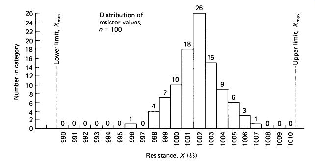
FIGURE 10-5 Distribution of sample data for Example 10-4.
than
delta_max = Es = 1.16 x 2.003 = 2.32 (10-8)
The upper 1% limit is nearer to the mean. We calculate the number of standard deviations to this limit:
Consulting Table 10-1, we see that the number of scores lying beyond 3.5 standard deviations from the mean in one direction is 0.00023 of the total. This means that we are 99% sure that not more than 0.00023 X 100,000 = 23 units per shipment will be out of tolerance in this direction. In the opposite direction, the limiting lies 990- 1001.87 _ 2.
32 standard deviations from the mean, and essentially no failures in this direction are anticipated. The results then establish a 99% confidence that the number of failures per 100,000 will be 23 or less, and it would seem unnecessary to undertake the expense of 100% testing.
Two worries haunt the manager who makes the decision of the foregoing example. First, we are assuming the population distribution to be normal. Figure 10-5 does not show any marked departure from the normal, so the assumption is reasonable, but we cannot be perfectly sure, especially at the tails where sample data are sparse. Second, the mean and deviation may change as the machine ages, new workers are put on the job, new batches of raw materials are used, and so on.
This makes it desirable that the sampling test be executed each month and that the samples be drawn after the month, s run is completed but before it is shipped, so that any changes on the line will be reflected in the sample.
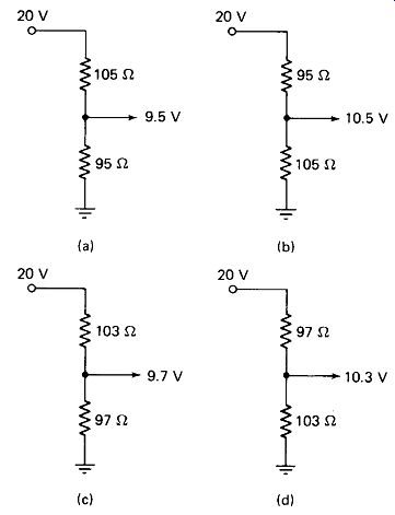
FIGURE 10-6 Voltage divider composed of two nominal 100-ohm 5% resistors:
worst-case analysis of minimum (a) and minimum (a) and maximum (b) outputs,
and statistical analysis with 99.9% confidence of minimum (c) and maximum
(d) outputs.
10.7 CUMULATIVE ERRORS
A component manufacturer’s tolerance specification generally takes the form of a guarantee that the components will not deviate from the marked value by more than the percentage specified. No information about the statistical spread of values within this tolerance range is implied, and we would have no grounds for complaint if a shipment of one thousand 100-ohm 5% resistors contained 500 that measured 95 ohm and 500 that measured 105 ohm.
Worst-Case Design assumes that the worst-possible combination of circuit values will eventually come up, and guarantees reliability in spite of it. To take a simple example, a voltage divider composed of two 100-ohm 5% resistors from a 20-V source could put out anything between 9.5 and 10.5 V, as shown in Fig. 10-6(a) and (b).
However, if we can determine that the actual distribution of component values is approximately normal, with the values occurring randomly, we may be able to employ a more economical statistical design technique.
Statistical design recognizes that the probability that the worst-case combination will actually occur may be so slight as to be negligible, especially where three, four, or more parameters must all go to their extreme limits together to produce the worst case. To understand why this is so, you must understand that cumulative probabilities multiply. For example, the probability of rolling a six on one die is 1/6.
The probability of rolling another six on a second die is also The probability of rolling a pair of sixes is therefore | X , or The probability of rolling four sixes with four dice is 5X£XiX5>0rdh- The point to be taken here is that four events, each of which has a fairly high probability of occurrence taken alone, have an almost negligible probability of occurring together.
Let us assume that we have used the method of Section 10.6 to determine that the 100-ohm resistors for our voltage divider are normally distributed with a mean of 100.0 ohm and a standard deviation of 1.5 ohm. The 5% limits each he 5/1.5, or 3.3, standard deviations from the mean, and Table 10-1 indicates that 0.00048 of the resistors will lie beyond the limits in each direction. Actually then, 0.00096, or about 0.1%, of the resistors will be rejects. Another way of saying this is that the probability that any one resistor will be at or beyond one of its worst-case limits is 0.00096. The probability that the other resistors will at the same time be at or beyond its other worst-case limit is the product 0.00096 X 0.00048, or about 1 chance in 2 million.
We can compute the probability of R, of the divider falling more than 2 standard deviations above the mean while R2 falls more than 2 below. From Table 10-1 the area beyond x/a = 2.0 is 0.0228, and the product of two such probabilities is about 0.05%. Of course, it is equally probable that R2 will be high while Rt is low, so we have a total probability of about 0.1% that one resistor will be 3 ohm (2 standard deviations) high while the other is 3 low. We are thus 99.9% confident that the voltage limits of the divider will be within 9.7 to 10.3 V, as shown in Fig. 10-6(c) and (d). It may be more economical to plan on ±3% tolerance for the output voltage and troubleshoot the 0.1% of cases where this limit is exceeded than to purchase precision resistors to ensure a worst-case limit of ± 3%.
Addition of Several Distributed Values: When a number of normally distributed component values are added (as in the case of series resistors), the mean and standard deviation of the total can be computed readily from the means and standard deviations of the components:
Where parallel combination is involved, resistance values can be converted to conductance values (G= 1 /R) and the conductance distribution determined from the foregoing equations.
EXAMPLE 10-5 Twenty-five 20-M0-ohm 5% resistors are connected in series to form a 500-MQ high-voltage probe for a 20-k0/V meter. The resistors are randomly selected and are normally distributed about a mean of 20 M ohm, with the 5% limit representing 3 standard deviations. What is the tolerance of the composite probe?
Solution
Extending equation 10-10 for 25 values of a, each equal to (5%X 20 M ohm)/3, or 0.33 M ohm:
Taking the tolerance limit as 3 a (yielding a 0.25% chance of being out of tolerance), the ohmic limits are ±3 x 1.65, or ±4.95 M ohm. This is a tolerance of ±4.95 MJ2 500 M-ohm This same technique can be applied to the subtraction of distributed values.
A batch of axles may be required to be randomly fitted into a batch of drilled holes.
If the distributions of axle and hole diameters are known, we can predict the probability that a clearance less than some specified value will be encountered.
Equations 10-11 and 10-12 now become
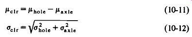
(10-11), (10-12).