PART II---INSTRUMENTATION AND SIGNAL PROCESSING
Electrical measurement
11.1 DEFINITION OF TERMS
In making measurements we employ a number of terms which need to be accurately defined if they are to be intelligently used.
Sensitivity: a measure of the smallest input signal that will produce an observable output (i.e., sensitivity 1 mV rms), often expressed as a ratio of output to input (i.e., sensitivity 100 mV rms for full-scale deflection of 100 divisions).
Accuracy: the degree to which the measured value approaches the true value.
Usually expressed as the percent error that may occur (i.e., accuracy ±5% of reading or ± 1.5% of full-scale value, whichever is greater). Sometimes expressed as the maximum amount of error that may occur (i.e., accuracy ± 0.05 V).
Precision: the degree to which a measurement is sharply defined, expressed approximately by the number of significant figures in the reading. If a four-digit digital voltmeter has a precision of ± 1 mV, we will be able to use it to adjust two power supplies to a reading of 5.000 V with assurance that they are no more than 2 mV different in voltage. If the accuracy of the meter is ±0.1%, the true voltage of the supplies will be sure to lie within the range 4.995 to 5.005 V.
Linearity: the degree with which a graph of the actual value of the quantity versus the reading of the indicator deviates from an ideal straight line between the end points of the actual curve. Actually, it is a measurement of non-linearity, calculated as follows:
normal linearity = max deviation of reading / full-scale reading (11-1)
Figure 11-1 provides an illustration of the properties of sensitivity, accuracy, precision, and linearity. There are many other definitions of linearity, the most common being independent linearity, in which the ideal straight line is adjusted for best fit to the actual curve, and zero-based linearity, in which the zero points are fixed together but the slope of the ideal line is adjusted for best fit.
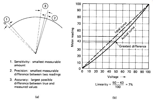
FIGURE 11-1 (a) Illustration of the definitions of sensitivity, precision,
and accuracy, (b) Illustration of the definition of normal linearity.
1. Sensitivity: smallest measurable amount
2. Precision: smallest measurable difference between two readings
3. Accuracy: largest possible difference between true and measured values
Hysteresis: the amount that a quantity can change before the measured value changes. Often expressed by the graphic words slop, stickiness, or dead zone.
Drift: the amount that a measured value (or a quantity) changes per unit time in the face of temperature, aging, or other variables. For example, an oscillator may be specified as follows: stability, ±20 Hz/h after 0.5-h warmup. A standard cell may be specified: stability, ±5 uV/yr.
11.2 ACCURACY OF ELECTRICAL STANDARDS
Electrical units were originally defined in terms of physical quantities in the CGS (centimeter-gram-second) system. For example, a coulomb of charge was defined in terms of the force (in g- cm/ ohm) between two plates held a certain distance (in centimeters) apart. With the technology that existed around the turn of the century such physical measurements were difficult to make accurately, so a system of international units based on direct electrical measurements was adopted. For example, the volt was defined in terms of a standard cadmium cell of precisely specified construction. The voltage produced by this cell was defined as 1.01830 international volts, and it was hoped that this voltage would prove to be the same as that derived by the CGS system. As technology improved, differences as large as 0.05% became apparent, and in 1948 the international system was replaced by the so-called absolute system, which was refined in 1960 to become the Systeme International (SI). A comparison of previous international units and the new SI units follows:
1 international coulomb = 0.99985 C (SI)
1 international ampere = 0.99985 A (SI)
1 international volt = 1.00034 V (SI)
1 international ohm = 1.00049 ohm (SI)
1 international watt = 1.00019 W (SI)
1 international farad = 0.99951 F (SI)
1 international henry = 1.00049 H (SI)
Accuracies on the order of 10 parts per million (0.001%) in voltage and other electrical units have been obtainable since the early days of electronics. Present standards are accurate to a few parts per million, and precise to better than 1 ppm.
Time can be measured to better than 1 part in 80 billion (8 X 10^10). These accuracies are obtained through painstaking work and are available only from primary standards maintained at government-operated laboratories, such as the National Bureau of Standards. Commercially available secondary standards and measuring devices are available with voltage and resistance accuracies on the order of 5 to 10 ppm. Time signals can be generated independently with accuracies much better than 1 ppm. Timing accuracies approaching that of the primary standard are readily available from the Bureau's radio station WWV, but no one has yet found a way to broadcast a standard volt.
11.3 MEASUREMENT TECHNIQUES
Whenever measurements that you have taken are of any importance, you may be sure that they will be challenged-by a rival within the company seeking to impress the boss at your expense, by a plant or government inspector, by a customer, or by a patent attorney. It is therefore of great importance that you acquire the habit of taking and recording measurements in a form that inspires confidence and stands up under scrutiny.
Format for Data: Every recorded measurement should contain an explanation of what the data refers to. The number 2800 scribbled diagonally across a scrap of paper will probably not impress an FCC engineer investigating an alleged violation.
The following format may carry more weight: 19 March, 1979, 9:30 A.M. Field strength of transmitter second harmonic measured with Acme test fixture at distance 200 ft N of tower. V2 - 2800 pV rms. John Doe This brings up several additional points. Every data record should be dated.
It is most frustrating to open a file and find two calibration charts for a test instrument, one of them obviously obsolete, but neither of them dated.
The instrument used in making the measurement should be identified, by serial number if several of the same type are available. This makes it possible to go back and check the calibration of the meter if your results are questioned. It also provides an indication of the degree of accuracy to be expected. A recorded value of 275 V dc (DVM) would be expected to be more accurate than a recorded value of 275 V dc (VOM).
Units should be included after each number recorded. Don't leave the milli- or micro- to be assumed, and always distinguish between rms, peak, and peak-to-peak measure of ac.
The person taking the data or preparing the chart should sign it. This tells the reader whom to see for more details and lends to the legal validity of the document.
Instrument Limitations: The accuracy specification of a meter is not the only limit on its performance. Manufacturers often omit any reference to other limitations, but you should check out your instruments on these points:
. What are the upper and lower cutoff frequencies on the ac ranges? Some VOMs and DVMs lose response above a few hundred Hz, while others are good beyond 100 kHz.
. Does your meter respond to dc components on its ac scales?
. Does your meter respond to the peak, average, or true rms value of a signal on its ac scales? Only special true-rms voltmeters provide valid readings for non-sine waves. Peak- and average-responding meters are calibrated with the rms equivalent for sine waves only.
. Does your meter respond to the peak or average value of an ac signal riding on a dc level on its dc ranges?
Measurement Pitfalls: Here are a number of tips for interpreting measured data:
. Meter accuracy is usually specified by allowable error as a percentage of full scale. Thus a reading of 35 V on the 100-V scale of a 3%-accuracy meter must be interpreted as having limits of 35 ± 3 V, or 32 to 38 V. We may acquire confidence that a particular meter does better than this by comparing it with a lab standard, but the manufacturer , s certification is limited to what in this case is a nearly 10% error.
. Meter calibration often changes abruptly with scale changes. A meter may show 2.45 V on the 2.5-V scale, and suddenly jump to an indication of 2.6 V when switched to the 10-V scale, without any actual change in the measured voltage taking place. Where a string of readings from 2.0 to 5.0 V is to be taken, it may be wisest to take all readings to the 10-V scale to avoid the disturbing jump in the curve at 2.5 V due to range change.
. Beware of subtracting two pieces of data. The uncertainty associated with each reading can make the result of a subtraction almost meaningless. For example:
90 V ± 3% minus 80 V ± 3% could be:
92.7 V - 77.6 V = 15.1 V, or at the other extreme:
87.3 V-82.4 V = 4.9 V
The nominal result is 10 V, but the limits of error are ±51%.
. The numeral 5 appears frequently as the last digit of measured data. If a meter pointer falls between 47 and 48 V, we may record the reading as 47.5 V. If a digital meter keeps alternating between 1020 Hz and 1019 Hz, the data may be recorded as 1019.5 Hz. If such data are later rounded off in the course of calculation, it would be unwise to always round the digit preceding the 5 to the next higher (or the next lower) integer, as this would tend to artificially bias the average of all the data one way or the other. The number 75 lies exactly midway between 70 and 80, and we should not arbitrarily bias our choice by rounding always to one or the other. A commonly accepted rule for rounding off fives is to round higher if the preceding digit is odd, and round lower if the preceding digit is even. This changes the odd numbers to even and keeps the even numbers even in the last digit of the rounded number. On the average, as many numbers will be rounded high as low, and the average of the data will be unbiased. Some examples of rounding fives from 4 to 3 figures follow:
4875 » 4880 3195 3200
4885 « 4880 3205 « 3200
11.4 THE DECIBEL SYSTEM
The decibel (dB) system of measure is widely used in the audio, radio, TV, and instrument industries for comparing two signal levels. There are two main points to remember in applying this system:
. A decibel measure is a ratio, not an amount. It tells how many times greater or how many times less a signal is compared to some reference.
. Decibel measure is nonlinear.
20 dB is not twice as much as 10 dB.
The original unit "bel" was defined as the logarithm (to base 10) of the power ratio of two signals. This unit proved too large, and was split into tenths, or decibels:
«dB = 10 1°g - df (11-2) where P] is the reference power (the input signal level, or perhaps an industry-wide standard-reference level) and P2 is the signal in question (the output signal). A little reflection, or a few moments with a calculator will reveal that a dB is always positive for a signal greater than the reference level, and always negative for a signal less than the reference level. Zero dB means equal levels-no gain, no loss. For reference, the transposition of equation 11-2 is given:

(11-3)
Choosing a log-based system allows a tremendous range of power ratios to be encompassed using only two-digit numbers, without sacrificing discernment at the low end of the scale:
1 dB = 1.26:1 power ratio 50 dB = 100,000:1 power ratio
The graphs of Fig. 11-2 illustrate this point. Both graphs show the same data.
Voltage and Decibels: Voltage' is much easier to measure than power, so it would be convenient to apply the decibel system to voltage measure. Since P= V1/R, and squaring a number is accomplished by multiplying its logarithm by 2, we can write equations 11-2 and 11-3 as:
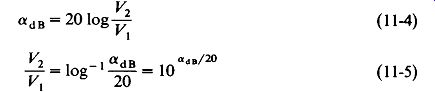
(11-4)
(11-5)
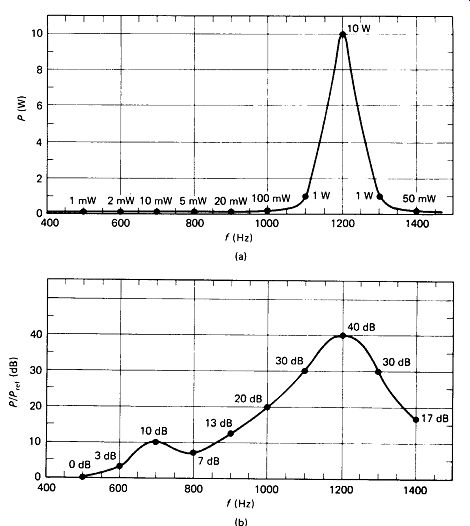
FIGURE 11-2 (a) A graph of power output versus frequency for a tuned amplifier
so compresses the power levels below 100 mW that they cannot be seen, (b) The
same data, converted to decibels with 1 mW-0 dB, shows all power levels clearly.
These equations rest on the assumption that R, for the reference voltage Vx is the same as R2 for the measured voltage V2. This restriction is often ignored in practice, but the results obtained thereby are not correct. If the impedance driven by K, is not known to be equal to the impedance driven by V2, the impedances must be measured, the two power levels calculated, and equation 11-2 applied. If the values of and R2 cannot be determined, the decibel system cannot properly be applied.
Decibel Standards: The audio industry has agreed upon a standard reference signal of 1 mW on a 600-ohm load, which equates to 0.775 V rms. Meters calibrated to this standard can only be read directly when used on a 600- ohm line. When used on other lines, the reading must be corrected as follows:
EXAMPLE 11-1 An audio meter reads - 4 dB across a 16-ohm speaker. What is the actual level? Solution The power error will be as the ratio of the 600-ohm standard to the 16-ohm measurement, since P - V1/R.
16 Expressed in dB, this ratio is a dB - 10 log P/P'
dB = 10 log 37.5 dB - 15.7 dB
This number of dB must be added to the reading:
x- -4+ 15.7-11.7 dB
The television industry sometimes uses a standard reference of 1 mV rms on a 75-ohm line.
Adding Decibels: Signal transmission in a large system involves multiplying by some factor Av each time an amplifier is encountered and dividing by a loss factor Fv each time a signal splitter, attenuator, or length of cable is encountered.
However, if all the system component voltage ratios (V0/Va,) were specified as decibels (positive for gain, negative for loss), we could determine the total system gain by algebraically adding the dB contribution of each component. This is because adding logs of numbers effectively multiplies the numbers, and subtracting logs effectively divides. This is often done in practice, because additions and subtractions are much easier to keep track of than multiplications and divisions.
EXAMPLE 11-2
Figure 11-3 shows a television master-antenna system, with the input signal expressed in dB (reference being 1 mV) and each component expressed by the dB ratio of its Vo/V . An attenuator is to be placed in the line to TV set 51 to provide a 10-dB signal level at the set. What size of attenuator should be used?
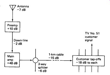
FIGURE 11-3 Example 11-2 Illustrates the advantage of decibel measure
In system work.
Solution
The signal level is - 7 + 10, or +3 dB out of the preamp, + 1 into the main amp, + 49 into the splitter, +43 out of the splitter, +28 into the customer tap-off box, and + 10 dB out of the tap-off. No attenuator is therefore required.
Anyone not yet convinced of the value of working in dB is invited to work Example 11-2 using voltage ratios. Use 450 /iV for the antenna signal, X 3.2 for the preamp, + 1.2 for the down line, X 260 for the main amp, -+- 2 for the splitter, -+ 5.6 for the 1-km cable, and +7.9 for the tap-off box. Shoot for a customer signal of 3000 fiV, and try to do it in your head.
Fast Decibel Conversions: People who work frequently with decibels soon commit the following table to memory. With it, any voltage ratio can be converted instantly to dB (or the reverse) without using a pencil or calculator.
To get values not listed in the table, just remember that adding dB is the same as multiplying voltage ratios, and subtracting dB is the same as dividing ratios.
EXAMPLE 11-3
Convert to voltage ratios: 26 dB, -55 dB.
Solution
26 dB - 20 dB + 6 dB
= 10 x 2 = 20 voltage ratio 55 dB = 50 dB + 6 dB - 1 dB
= 316 x2 -+- 1.
12 = 564 voltage ratio
The minus sign simply indicates a level 564 times below the reference, which we may wish to express as 1 /564 voltage ratio.