14.1 DEFINITION, CLASSIFICATION, AND SPECIFICATIONS
A transducer is a device that changes energy from one form to another.
In electronic instrumentation we are most often interested in changing some physical quantity such as heat, light, or motion into electrical energy for measurement, recording, or processing.
Transducers may be active, in which case they will generate an electrical signal without the application of external voltage or current, or they may be passive, in which case they will require excitation by an external voltage or current.
Transducers may produce an ac or a dc output signal, and often in the case of passive types, this depends on whether they are excited by ac or dc.
The simplest transducers' to use are the voltaic and resistive types, which produce a voltage change or a resistance change in response to a change in some physical property. More difficult in application are transducers that produce a change in capacitance or inductance in response to physical properties.
For any transducer, there will be three primary concerns about its suitability of operation.
1. Sensitivity: This is expressed wherever possible in terms of output voltage change per unit input-property change. In measuring temperature, it would be /iV/ ° C, or for displacement, V/cm. For some transducers it may have to be expressed in terms of resistance, inductance, or capacitance change per unit physical property change (i.e., 2.3 pF per lb/in.^2 change in pressure for a nominal 120-pF unit).
2. Linearity, Offset, and Dynamic Range: Ideally, it would be nice to have a transducer that generated zero voltage at absolute zero temperature, and 1 mV for every °C above that, up to and beyond 1000 mV at 1000°C. Few transducers even approach this ideal. Offset (nonzero output for zero input) can be handled easily by the techniques of Section 19. Dynamic range generally depends upon material selection and physical structure. Nonlinearity of the input-output curve is a persistent problem, and quite a game can be made of trying to linearize an inherently nonlinear transducer. Solutions may involve anything from simply compressing the meter scale at one end to complex microprocessor programs providing four-digit readout.
3. Noise Immunity; Noise is defined as anything other than the desired signal. If a pressure transducer is affected by temperature, or if a light-intensity transducer is affected by nuclear radiation, you have a noise problem.
14.2 TRANSDUCER TYPES
Literally hundreds of transducer types exist, and the technician must become accustomed to an occasional surprise at the clever way someone has devised to sense some physical property. A relatively few types serve as the workhorses of the industry, however, and we will concentrate on descriptions of these.
No attempt is made to classify the devices by function, as this tends to limit rather than expand their range of application. A microphone is not listed as an audio transducer, because with suitable circuitry it can be used to measure the time between two impacts, thus measuring distance, velocity, or density.
Switches are the most common transducers because they are inexpensive and easy to understand. They are commonly applied as:
. Limit switches, to indicate end of travel on elevators, garage-door openers, machine-tool bits, and so on. Two switches may be placed in line, the first indicating slow down, and the second halt. Magnets may be used to actuate the switches if physical contact is undesirable.
. Liquid-level indicators when attached to a float.
. Pressure indicators when attached to a bellows or piston-against-spring assembly, as in Fig. 14-1(a).
. Temperature indicators when attached to a bimetallic strip, as in Fig. 14-1(b).
. Rotational speed indicators when activated by centrifugal force.
Variable Resistors are often geared to a linear moving element or simply structured as a linear slide wire to provide continuous position readout. They are also formed as a nest of loose-packed carbon granules so that resistance decreases when pressure on a plug packs them closer together. This is the basis of the familiar telephone microphone.
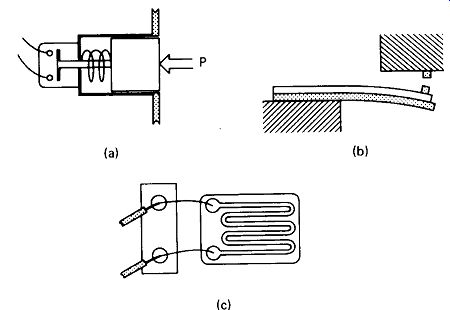
FIGURE 14-1 (a) Pressure-sensitive switch, (b) Switch operated by a temperature-sensitive
bimetal strip, (c) Strain gage with terminal mounting block.
Strain Gages are most commonly made by etching thin conductive paths of metal on a flexible insulative backing. They are then bonded to a structural element (usually metal) that is placed under mechanical stress. The very slight elongation of the metal stretches the conductors, increasing the resistance of the gage by something on the order of 0.01% for typical stresses in steel. If a strain gage of unknown properties is connected as one arm of a Wheatstone bridge, the variable dial can be calibrated in terms of stress (load in kg/cm^2) for the metal being tested.
Figure 14-1(c) shows a strain gage with a terminal block bonded in place to keep the relatively heavy instrument wires from tearing up the delicate strain gage.
Strain gages made from semiconductor materials are available with resistance changes on the order 100 times that attainable with metal gages. Temperature sensitivity and nonlinearity have limited the popularity of these gages.
Thermocouples are composed of a simple junction between two dissimilar metals, usually a welded lead enclosed in an inert protective tube. A small voltage which increases with temperature appears across the junction. Typical thermocouples operate up to 3000°F (1650°C) and generate a few tens of millivolts. Iron-constantan thermocouples, for example, generate about 32 mV at 1000°F (538°C).
The output of a thermocouple can be measured directly with a sensitive galvanometer, but voltage drop across the relatively high resistance of the thermocouple wire limits the accuracy of this technique. Some form of self-balancing potentiometer with electronically amplified null detection is generally used. Figure 14-2 shows a thermocouple-potentiometer circuit, and points up the fact that the junctions of the thermocouple wires to the measuring instrument form two additional thermocouple junctions whose voltage must be taken into account.
These voltages will be relatively small but will vary with ambient temperature changes. Where highest accuracy is required and some inconvenience can be tolerated, a reference junction held at 0°C by a bath of melting ice can be employed.
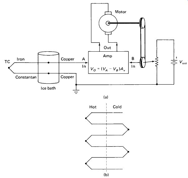
FIGURE 14-2 (a) Thermocouple feeding a self-balancing potentiometer, (b) Thermopile.
Undesired thermoelectric voltage generated across dissimilar metals at sockets or connectors is often the cause of thermal instability in sensitive dc amplifiers. A series of thermocouples, called a thermopile, can be used to obtain higher output voltages, as shown in Fig. l4-2(b). Notice that each hot junction necessitates a cold junction and two wires leading to it. Thermopiles using semiconductor rather than metal elements have been used with some success as direct heat-to-electric power converters.
The Peltier cooling effect should also be mentioned at this point. If a relatively high current is passed through the junctions in Fig. 14-2(b), one set of junctions will be heated and the other will be cooled. This effect has been used to provide spot cooling of critical elements in densely packed equipment without the bulk and moving parts of conventional refrigeration techniques.
Thermistors are resistive elements whose resistance decreases with increasing temperature, in some cases by as much as - 7%/° C.
Thermistors are available with 25°C resistances from less than 1 to several M- ohm and with operating ranges from - 80 to + 1000° C.
Physical shapes and sizes vary widely, from beads of 1-mm to discs of 25-mm diameter.
Thermistor curves are inherently nonlinear, as shown in Fig. 14-3, but special three-terminal networks (composed of two thermistors and two resistors in a single package) are available which provide a nearly linear voltage-versus-temperature output over moderate ( - 30 to + 100 ° C) temperature ranges.
Thermistors are most commonly employed in a Wheatstone bridge or voltage divider circuit for temperature measurement and control, in which case the IV product must be held to a minimum to prevent self-heating. Deliberately raising the IV product to produce self-heating allows the thermistor to be used to measure other parameters that act to carry away heat. Examples are wind or air-flow velocity, level of immersion in a liquid, viscosity of a liquid, and R value of a thermal insulator.
Thermistors are also used for temperature compensation in electronic circuits.
As an example, the thermistor in Fig. 14-3(c) lowers the transistor’s bias point at high ambient temperatures, limiting its collector dissipation to a safe value.
Finally, thermistors can be used to produce time delays from less than 1 s to several tens of seconds by operating them in the self-heat mode and taking advantage of their thermal mass, which delays warmup and consequent resistance drop.
Photodetectors are available in a rather bewildering variety. Primary factors for comparison are sensitivity and response speed. Other factors are temperature sensitivity, bulk and fragility, cost, and spectral response peak (some devices respond better to red or infrared or blue or ultraviolet). We will list the five most common photodetectors in order of increasing response time.
. Photomultipliers (Fig. 14-4) are high-vacuum glass tubes requiring a thou sand-volt-level power supply. However, they have a response time on the order of 1 ns and a sensitivity to low light levels which is several times better than the best solid-state detectors. They contain a cathode which emits electrons when struck by light, and a series of plates at successively higher positive potentials, to which the electrons are attracted in turn. At each plate the impacting electrons splash up additional electrons, so the total electron current builds up.
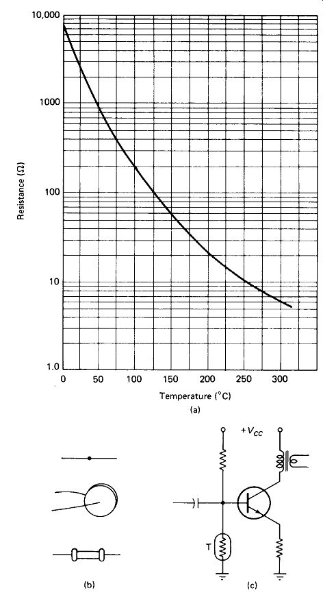
FIGURE 14-3 Thermistors are temperature-sensitive resistors: (a) typical R
versus T curve; (b) typical thermistor packages; (c) thermistor used to bias-stabilize
a power-transistor amplifier
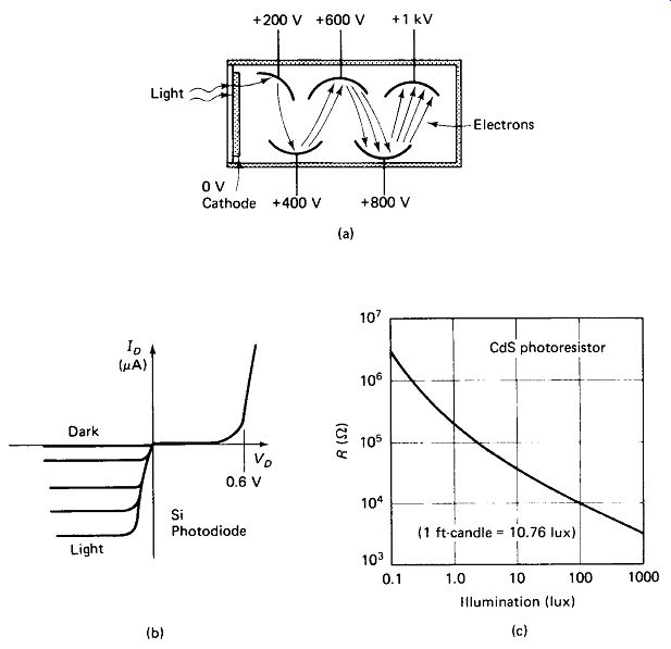
FIGURE 14-4 (a) Photomultiplier-tube structure, (b) Silicon-photodiode characteristics.
(c) Typical CdS photo-resistive cell characteristics.
. P-N and PIN silicon photodiodes have response times on the order of 20 ns and 2 ns, respectively. Under forward bias they behave much like conventional diodes, but their reverse leakage current increases with light intensity due to formation of hole-electron pairs near the junction. Currents of 10 uA are typical under room light. The PIN photodiode has a layer of intrinsic (pure) silicon between the P- and JV-doped regions to reduce dark-current leakage and junction capacitance.
. Phototransistors, in which base current is replaced by light-generated hole-electron pairs, have response times on the order of 2 us and collector currents of a few mA at room-light levels. The base lead is usually brought out so the transistor can also be turned on in the usual manner. Light activated SCRs (LASCR) have similar response times. Photo FETs are somewhat faster, with response times in the vicinity of 0.1 us.
. Silicon solar cells are large-area P-N junctions which produce direct current when struck by light. Conversion efficiency in sunlight is about 10%. A typical cell produces 0.4 V output and provides about 5 mW/cm2 under bright sunlight. Response times are on the order of 5 us.
. Resistive photocells of cadmium sulfide (CdS) and cadmium selenide (CdSe) are very popular because of their low cost and relatively high voltage and current capabilities (250 V and 300 mW typical). However, they are extremely slow, exhibiting response times on the order of 1 s at low light levels, down to about 10 ms at bright room-light levels. A wide variety of types with on resistances down to the 100-ohm range are available.
Piezoelectric Crystals such as quartz and barium titanate produce a voltage when placed between two electrodes and subjected to mechanical vibration. The voltage is proportional to rate of change of force, so only dynamic forces are recorded. The piezoelectric effect is the basis of the common crystal and ceramic microphones and phonograph pickups and is fairly widely employed in the measurement of vibration and shock. Output voltages from 1 to 100 mV, depending on sound level, and source impedances of approximately 50 k-Ohm are common for crystal micro phones.
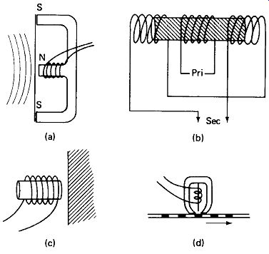
FIGURE 14-5 Magnetic transducers: (a) dynamic micro phone and headphone principle;
(b) linear variable differential transformer; (c) proximity detector; (d) magnetic-tape
pickup.
Magnetic Transducers take a variety of forms, some of which are shown in Fig. 14-5. The common feature is that the air gap of a coil’s magnetic core is varied by mechanical displacement, resulting in a change in inductance of the coil. In some cases, such as the magnetic headphone of Fig. 14-5(a), the coil is self-excited by the field from a permanent magnet, so that a voltage is produced when air vibration on the diaphragm changes the air gap. In other cases the coil is excited externally. The two secondaries of the linear variable differential transformer (LVDT), Fig. 14-5(b), are connected in series reverse phase, so that, with the movable core centered, the output voltage is zero. Moving the core produces an output in or out of phase with the primary depending on direction of motion. The proximity detector of Fig. 14-5(c) is used in metal detectors and vibration monitors. It is used as the inductor in an LC oscillator at a relatively high frequency (above 100 kHz) so that an inductance change of less than 0.01% will produce a measurable change in oscillator frequency. Figure 14-5(d) gives a brief sketch of a magnetic-tape-player pickup head. Variations in reluctance of the magnetic coating on the tape produce variations in the inductance of the pickup coil as the tape moves past the head gap.
Generator Transducers: Small rotating generators with a permanent-magnetic field are often used as transducers. They produce an output voltage (generally dc) which is directly proportional to rotational speed. Driven by small turbines or rotating vanes, they can be used to measure wind or fluid-flow velocity.
Radiation Transducers: The high-energy radiation associated with nuclear activity is capable of ionizing (stripping away an electron from) the atoms it impinges upon. The Geiger-Muller radiation counter (Fig. 14-6) contains a low-pressure gas and an anode at a very high positive potential. Entering radiation ionizes a single particle of the gas, but the resulting two ions quickly collide with and ionize other gas atoms as they are accelerated by the high potential between the anode and cathode. Thus each entering particle of radiation causes complete ionization and conduction within the tube, regardless of its relative intensity. The ionized condition lasts about 1 ms, so the count rate of the tube is limited to about 1000 per second.
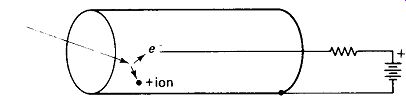
FIGURE 14-6 Geiger-Muller tube structure.
Capacitive Transducers: Changes in capacitance can be produced by varying the plate spacing, dielectric constant, or plate area. Readout can be accomplished by measuring the change in ac current as reactance changes, by sensing the change in voltage across a charged capacitor as its capacitance changes (V= Q/C), or by measuring the frequency of an oscillator controlled by the capacitor transducer.
Figure 14-7 shows some of the possible applications: (a) a paint-thickness gage, (b) a capacitor microphone, and (c) a dielectric-constant sensor to detect which of two liquids is flowing in a pipe.
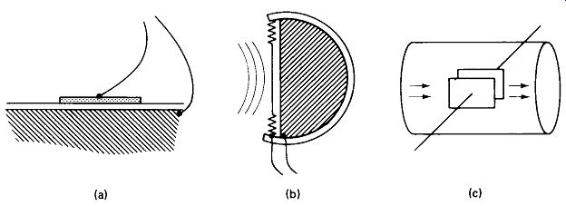
FIGURE 14-7 Capacitive transducers: (a) paint-thickness gage; (b) capacitor
microphone; (c) liquid-dielectric sensor.
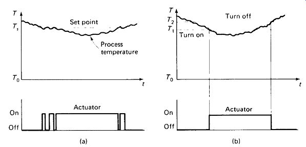
FIGURE 14-9 (a) Random fluctuation of the sensor output can cause chatter
of the actuator near the set point, (b) Introduction of a hysteresis or dead
zone between turn-on and turn-off eliminates chatter.
14.3 FEEDBACK CONTROL SYSTEMS
The usual automobile heater is an open-loop system: we turn it on, pick a setting, and hope for comfort. If our choice is wrong, we readjust the setting. When we come off the expressway into the city, heating requirements change and again we adjust the heater manually. By contrast, the usual home heating system is a feedback or closed-loop system. We choose a setting on a calibrated dial, and the thermostat leaves the furnace on until that set point is reached. Variations in heating demand due to opened doors or outside temperature drop are handled automatically because the sensing device (thermometer) constantly measures the process variable (room temperature) and compares it to the demand point (thermostat setting). If the measured variable is below the demand point, the controller (thermostat switch) turns on the actuator (gas or oil valve) to restore the process variable to the demand point. Figure 14-8 illustrates this basic feedback control loop for an industrial heat-treating furnace. If the sensing device is a simple switch actuator (such as the bimetal strip used in most thermostats) there need be no electronics involved, but more advanced control systems use an electronic sensing device and a potentiometer or Wheatstone Bridge to produce an error or difference signal between the set point and the process variable. An amplifier is then used to allow the difference signal to control the actuator.
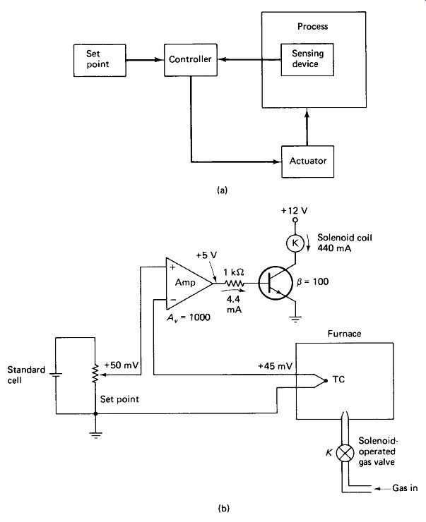
FIGURE
14-8 (a) Basic feedback or closed-loop control of a process. (b) Implementation
of feedback control for a gas-fired furnace with a thermocouple for a sensor,
battery and pot for set-point determination, amplifier and transistor coil
driver for controller, and solenoid gas valve for actuator.
14.4 PROBLEMS WITH FEEDBACK CONTROL
Dead Zone or Hysteresis: In general, two-position actuators such as switches and solenoids should be snapped from one position to the other and not "mushed" or " jittered" back and forth. This requires a certain small dead zone between the on and off switching points to screen out noise and irregularities in the transducer output, as shown in Fig. 14-9. Many actuators have hysteresis built in. For example, a relay that pulls in at 100 mA may not drop out until 75 mA, providing desired snap action automatically. In many cases the dead zone is provided by an electronic snap-action switch called a Schmitt trigger. The dead-zone requirement places a limitation on the precision attainable in the control of the process.
Response Time: The time a control system requires to respond to a change in set point or a change in the process requirement is generally of considerable importance.
If we change the demand temperature of our furnace from 200 to 250°C, we would like the new temperature to be reached as quickly as possible. Similarly, if we cause a temperature drop by opening the door and inserting an ingot of cold metal, we would like the temperature restored to its set point as soon as possible. Response time depends primarily upon the ratio of process inertia (in this example, the thermal mass of the furnace and its contents) to the strength of the actuating force (in this case, the Btu/h rating of the burner). Figure 14-10 shows the response times of two furnaces with different-size burners.
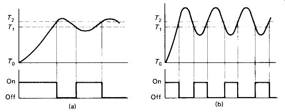
FIGURE 14-10 Improving response time generally aggravates the tendency to
overshoot and oscillate: (a) slow response, moderate overshoot; (b) fast response.
excessive overshoot.
Oscillation and Overshoot: The temperature of our heat-treating furnace is always oscillating between the turn-on and turn-off limits, which define the dead zone of the controller. In addition, there will be some overshoot and undershoot beyond these limits which will increase as response time is decreased. A well-insulated furnace with a small heating element will experience temperatures that rise and fall slowly, and there will be little overshoot, as shown in Fig. 14-10(a). However, if a larger heating element is used to reduce response time, as in Fig. 14-10(b), the temperature within the furnace is likely to rise considerably above the set point as heat spreads from the area of the burner to the area of the sensing device, even after the burner has been shut off. Attempts to increase response time in general have a tendency to increase overshoot and oscillation. Overshoot and undershoot can easily span a range much greater than that of the dead zone itself. If this is the case, attempts to increase the precision of control by narrowing the dead zone will be fruitless.
14.5 ADVANCED CONTROL TECHNIQUES
Overshoot Compensation: A clever and widely used technique for practically eliminating overshoot is illustrated in Fig. 14-11. The basic idea is to reduce the set point slightly whenever the heater comes on. The heater is thus shut off slightly before the process reaches the original turn-off point, and overshoot carries it to precisely the desired point. From then on, it is the set point that oscillates around an almost fixed process temperature. For maximum stability the depression of the set point must exactly equal the overshoot of the process, so the controller compensation must be adjusted to match the system. Changing loads (100 kg versus 1000 kg of ingots in the furnace) and changing activating forces (gas-pressure changes) will require a reset of the compensation control if oscillation is to be minimized.
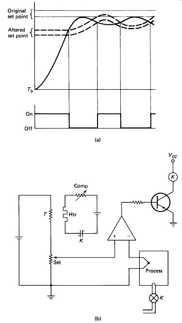
FIGURE 14-11-- Overshoot can be minimized by bringing the set point down to
meet the process coming up: (a) graphical analysis; (b) circuit implementation.
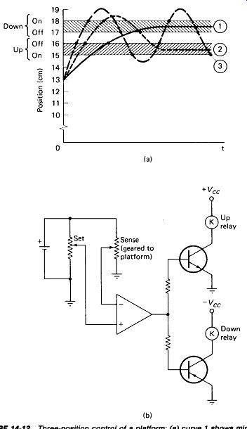
FIGURE 14-12 Three-position control of a platform: (a) curve 1 shows minimal
overshoot, curve 2 shows overshoot severe enough to activate the down relay
to return the platform to the set zone, and curve 3 shows severe overshoot
and undershoot resulting in continuous oscillation; (b) circuit implementation
of three-position control.
A common way to achieve set-point reduction is to use a thermal-sensitive resistor as part of the potentiometer or Wheatstone bridge circuit. This resistor is heated by a separate resistive element which is controlled along with the actuator.
A variable resistance in series with the heater controls the degree of set-point reduction. The response time of the heater-thermistor pair should approach that of the process itself if cancellation of process oscillation is to be achieved. Thermal mass may be added to the thermistor to lengthen its response time.
Three-Position Control: The controllers we have discussed thus far have been two-position controllers, the two positions being ON and OFF. Some control systems, however, obviously require three positions. In the case of an elevator they would be UP, OFF, and DOWN. For a hydraulic cylinder they would be EXTEND, HOLD, and RETRACT. Even inherently dynamic processes like the heat-treating furnace can benefit from three-position control. Imagine a large quantity of 500° C metal being thrust into a furnace set for 300°C. It may be desirable to employ a fan or cooling-water pump to bring the temperature more quickly back to the set point.
Oscillation of a violent sort is a common problem in three-position control systems. Figure 14-12 illustrates the situation using the example of a motor-operated vertical-positioning platform. The sensing device is a slide wire which forms one arm of a Wheatstone bridge. The platform is commanded to move up from its 13-cm initial position to a nominal 16.5-cm position by a rotation of the SET POINT potentiometer. The up relay turns on and the platform moves up. At 16 cm the up relay turns off, but because of its inertia, the platform does not come to rest until 17.5 cm (curve 1).
Now if the inertia of the platform were a little greater, or the speed of travel a little higher, the platform might overshoot to 18.5 cm, turning on the down relay, resulting in a reversal of the motor and a final rest point of perhaps 15.5 cm (curve 2). Notice that any rest point between the down on and up on limits is possible, depending upon the motor speed, platform load, and direction of approach. In the example, this is a span of 3 cm, which is likely to be objectionable.
The obvious solution is to increase the gain of the amplifier. A factor-of-10 gain increase would reduce the span of possible rest positions to 0.3 cm. However, this would greatly aggravate the overshoot problem, and it is likely that both overshoot and undershoot would exceed the down on and up on limits, resulting in continual reversals of the motor and oscillation of the platform up and down over a range far exceeding the 0.3-cm neutral zone, as illustrated in curve 3. These oscillations can be eliminated by slowing the system response time down (by a factor of 10), thus reducing inertial overshoot to a point where it remains within the 0.3-cm neutral zone, but such a slow response time may itself be objectionable.
The remainder of this section is devoted to resolving this dilemma: How can we build a control system with both minimum response time and minimum neutral zone, while avoiding the oscillation or " hunting" of the process variable which the attempt seems always to produce?
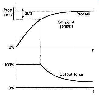
FIGURE 14-13 In proportional control the restoring force is proportional to
the deviation from the set point within the proportional band.
Proportional Control: If the amount of actuator force is continuously variable and is made proportional to the difference between the set point and the sensed process point, a system is produced which brings the output quickly toward the set point when the deviation is large, but slows down the approach as the set point is neared, as illustrated in Fig. 14-13. The actuator cannot be a relay or a solenoid in proportional control; it must be a continuously variable device. Most commonly, the actuator is an SCR or triac circuit, or a power transistor.
Proportional control often results in an objectionable offset between set point and process rest point. Offset is a function of process load and actuator force. In addition, mechanical systems have a hysteresis or dead zone caused by friction.
The deviation of the process from the set point can be reduced by increasing amplifier gain, but with the same risk as before: overshoot and oscillation.
The term proportional band has been coined to express the gain of a proportional control system. It is defined as the change in transducer output as a percent of full scale required to produce a 100% change in actuator output. In effect, it represents the deviation from the set point at which the output force begins to drop. Notice from Fig. 14-13 that the output force remains at its maximum until the process reaches 70% of its set point, whereupon it begins to decrease. If the set point is at full scale the proportional band is 30%. Smaller proportional bands reduce offset and hysteresis error, but tend to cause overshoot and oscillation.
Reset or Integrating Control is added to proportional control to reduce the offset and hysteresis errors. In this system the output force is proportional to the deviation from the set point plus the integral (accumulation over time) of that deviation. Thus a small error persisting over a long time will eventually build up enough output to move the process to a new rest point. Certain elevators are commonly seen to stop with a floor-leveling error of a centimeter or two and then resettle after about a second as a result of this action.
Rate Action or Derivative Control is added to proportional and reset control to decrease settling time and minimize deviations caused by upsets in system load. It operates within the proportional band to add an output force that is proportional to the negative rate of change (derivative) of the process variable. The output is thus reduced as the set point is approached, allowing the system to be operated with a smaller proportional band without excessive overshoot. In addition, an externally caused upset in the process, if it is fairly rapid, will produce an immediate and strong response from the controller, without waiting for the process to reach the limits of the proportional band.
Figure 14-14 shows the proportional, integral, and derivative outputs for a controller bringing a process from zero to a set point, and readjusting for an externally caused upset. The proportional band is about 40%. Integral and derivative outputs are limited to 10% and 40% of maximum proportional output, respectively. Notice that there is a small offset from the set point until the integral output builds up enough to reset it.
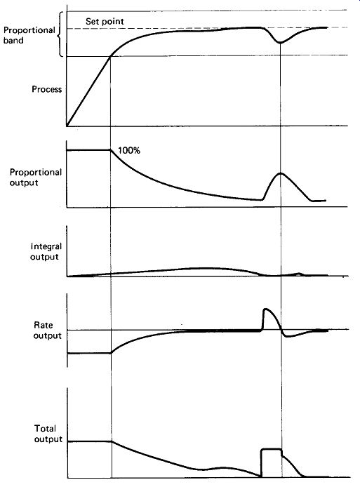
FIGURE 14-14 Proportional plus integral plus rate-action control brings a
process more quickly to the set point without overshoot or offset, and corrects
more quickly for process upsets.
Cascaded Controllers: It is sometimes advantageous to sense one or more secondary variables connected with a process in order to more effectively control the primary variable. In the furnace example, gas-line pressure might be sensed by a secondary controller whose output would be used to modify the overshoot compensation in the primary controller for continued minimum overshoot. The weight and temperature of the ingots arriving on the conveyer might be sensed by a third controller whose output would modify the demand point in anticipation of this external upset, thus keeping the process nearer the original set point. Such controllers are said to be operating in cascade.
Computed Control: The advent in the late 1960s of environmentally rugged minicomputers in the $10,000 price range made the application of computers to large control systems commonplace. Single-chip microprocessors in the $100 price range became available in the late 1970s, and brought computed control to small systems and even to individual instruments. The behavior of a computerized control system depends not so much on its structure or wiring as on the program that is loaded into it. Therefore, it is impossible to be specific about the actions of computerized controllers. Several general advantages can be pointed out, however.
1. Computerized controllers can be programmed to consider the history of a process as well as its current state. A sheet-steel-rolling process might then adjust the temperature and pressure at the second set of rollers based on the results achieved at the first set.
2. Programs can contain decision points altering the action taken or jumping control to an entirely different program. A bank of elevators can have separate programs for up traffic peak, day operation, down traffic peak, evening standby, and emergency evacuation.
3. Computers can handle more complex routines, including sequences and mathematical computations. One good example is transducer linearization, where a nonlinear device such as a thermistor is linearized by means of a lookup table or conversion program stored in memory.
4. Computerized controllers can scan a multiplicity of inputs--literally dozens in 1 ms--to take a variety of factors into account. A furnace controller might monitor temperature at six different places, gas pressure, air flow, temperature, and humidity, incoming ingot weight and tempera ture, and length of time the door is open-incorporating all of these factors into the control program.
5. Computers can handle several processes at once. A microprocessor in an automobile could control ignition timing and duration, carburetion, non skid braking, transmission shifting, and passenger environment, and still have time to play spelling games with the kids in the back seat if we wished to so program it.
6. Control programs can be easily modified. Adding a step to a process or meeting a new environmental or safety spec is usually a simple and inexpensive matter of changing a program memory chip rather than buying a new controller or rewiring the old one.