An adequate knowledge of basics can be of great help in understanding unfamiliar new circuitry and troubleshooting if in the absence of adequate service data. Here is a review of all the ac theory you once learned but have forgotten.
by Stan Prentiss
-----from an unpublished book "Today's Electronics--Electronics for Troubleshooting," by Stan Prentiss
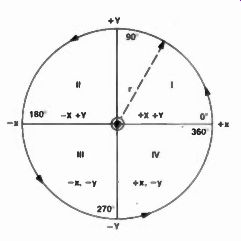
Fig. 1b The four quadrants and their positive and negative coordinates.
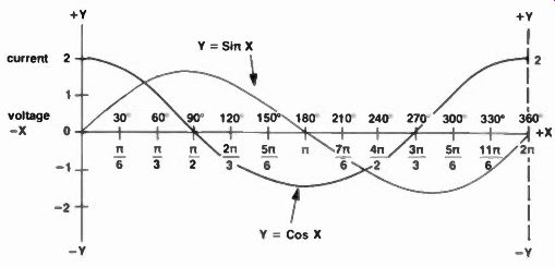
Fig. 1a A single cycle of alternating current (sinewave) showing y as (I)
x for both sine and cosine functions. Pi always equals 180°. An example also
of current leading voltage in a capacitive circuit.
Inductors, capacitors, transformers, and coupling-shaping networks, together with voltage dividers, form a very large segment of all electronics.
Dc voltage and current are the motivators and operators for every conceivable simple network. In this you will see that capacitors and inductors have certain effects on both direct current and alternating current in signal transmission/reception. That is the elementary difference between plain electricity and the more sophisticated electronics. Both come from the Greek word elektron, meaning amber. ... And amber, when rubbed with certain fabrics and other materials, attract light particles of wood just as a comb will attract paper Later, it was discovered by Ben Franklin and others that there are both positive and negative electricity that attract unlikes and repel likes, and these are now called electrons and protons, for negative and positive charges. In semiconductors, the charge carriers are currently identified as electrons and holes (a lack of electrons). As a further refinement, electricity can be considered in terms of work; and work means power.. . P = El. Electronics uses this energy and power to deliver or receive information by wires, circuits, air, space, through the oceans, or by special radiation such as laser beams. As money is a medium of exchange, so electronics is a method of intelligence transmission.
Satellites, radio, CB, 2-way communication and television are the world's outstanding examples.
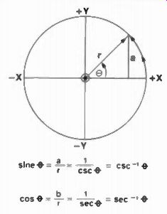
Fig. 2 Radius vector rotating about its (0) origin generates a unit of angular
velocity.
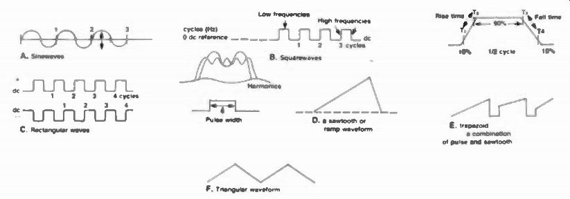
Fig. 3 Sine, square, pulse, ramp, trapezoidal and triangular waveforms all
play a part in signal processing.
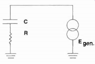
Fig. 4 A series RC circuit will charge and discharge at its RC time constant.
Alternating current
Almost all of the house or manufacturing current used in America today is delivered to us as alternating current (ac); and most electrical audio and video energy we hear and see arrives at receiver decoding circuits also as sinusoidal information in the form of signals whose waveshapes alternate above and below a zero reference line that is often referred to dc, to differentiate from positive or negative, or as simply a starting point. In Figure 1a, this alternation or sinusoid is drawn in the shape of a sinusoidal waveform, or what we commonly refer to as a sinewave. There are, of course, square, rectangular, triangular, sawtooth, trapezoidal waveshapes of all sizes and time durations, and we will discuss these also; but our main concern at the moment is with the all important sinewave, because that's the foundation for everything that follows.
This sinewave travels through an arc of 360 degrees, marked off in 30 degree sections (increments). As you see, it is also described in terms of radians where circular arc lengths are equal to the circle's radius. As you may remember from trigonometry, there are 57.295 degrees in one 360/ 2 pi t radian, and n radians amount to 180 degrees. Any angle, of course, can be converted from degrees to radians by putting it over 180 degrees and producing the answer as a fraction of n radians. For instance 20°/ 180° = n /9 radians. The rest of the degree-radian table in Fig. 1 a is calculated in exactly the same manner. Fig. 1 b illustrates the counterclockwise travel route the sinewave travels beginning at 0 degrees and continuing through 360 degrees_ As it passes through each quadrant, the signs for the X and Y coordinates change as shown. The sine (y = sin X) and cos (y = cos X) are identical except there is a 90 degree phase difference between the two ... a most important relationship when the normal quadrature (90 degree) phase angle between current and voltage in inductive and capacitive reactances is considered.
The two single cycles of alternations in Fig. 1 a, of course, are dual curve plots of the same sine and cosine functions--the sine curve beginning and ending at zero, and the cosine curve being a unit mark identified at Y point 2 as one fourth cycle advanced over the sine function. Shortly you will see that one of these curves can represent voltage and the other current as we come to grips with reactances. Were we discussing pure resistances, the sine and cosine alternations would be superimposed on one another, since across pure resistances, current and voltage are always in phase.
The angular velocity of such a sine/cosine wave is also worth knowing because it represents the speed with which the radius vector r is turning about the center origin to generate the angle theta. With repetitive rotation, angular velocity is ordinarily measured in radians/second (radians per second), and this amounts to a repetition rate, or an established (constant) frequency. So the angle theta can now be expressed as a function of time and the number of radians the radius vector must pass in any period of time. Therefore, two fundamental ac equations have been developed that you must remember for all time-and never forget!
1. (1.) (the angular velocity in radians/ sec) = 2 f, or 2 x 3.1416 f where Pi (3.1416) is derived from dividing 180°/ 57.295° in 1 radian, with the sweep through an angle or 360 degrees every 1/f seconds, or 2 radians.
2. 8 = w t... representing the complete angle resulting from rotating a radius in t seconds at an angular velocity of radians. So 0 could also equal 2 n ft.
In alternating current, the tangent, cotangent, secant, and cosecant functions are not used because, although they represent periodic events, their curves are not continuous throughout an entire cycle.
However, in vectors such applications are essential.
In Figure 2, the sine and cosine of 0 and their inverses-the secant and cosecant-are illustrated along with a unit of angular velocity. If you want to know the Y value at any point in either Figures 1 or 2, it amounts to: 6Y = r sin 6 ... since Y is proportional at all times to the sine of the angle times the length of the radius vector.
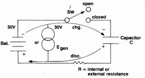
Fig. 5 A battery or a signal source may charge a capacitor
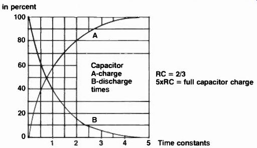
Fig. 6 Current/voltage value curves in exponential A, charge, and B, discharge,
RC times of capacitors.
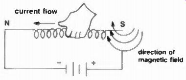
Fig. 7 An air core coil when held in the left hand, shows direction of both
current flow and magnetic field.
Waveforms
Of course, every video and audio waveform -be it voltage or current -is not simply a perfect sinewave: far from it! There must be variations, and these can be produced by changing amplitude (height) as well as frequency (duration), so that each pulse or curve of current can develop a voltage across some resistance/ impedance viewable on a video screen or audible through a loudspeaker. As this article unfolds, you will learn how one waveshape can generate another waveshape that's related, but totally different, just because certain reactances at specific frequencies behave the way they do.
There are subsonic frequencies below about 20 or 30 Hz (Hertz), sonic frequencies between about 30 Hz and 15,000 Hz that can be heard by those with excellent hearing (others only hear to about 12 kHz), and supersonic frequencies above 15 kHz that animals may hear for a period, but then lose. By contrast, the eye can easily see frequencies much lower than 15 cycles and, indeed, even millions of Hz (cycles), if it is properly presented in some sort of visible trace. The color spectrum, for instance is between 400 and 700 nanometers, and this translates roughly to between 3 x 10¹⁴ and 3 x 10¹⁵ Hz, an astonishing range since the nanometer is equal to one billionth of a meter, or 1/25,000,000 of an inch.
So, 400 nanometers amounts to 1/ 62,500 of an inch, while 700 nanometers become 1/31,500 inch.
Obviously, the higher the frequency, the shorter the wavelength. At 460 nanometers we see blue, green at 500, yellow around 590, orange at 600, and red from 630 to 780 nanometers. Of course, red, blue, and green then combine to form white which, in Y additive, R-Y, B-Y, G-Y, color television is known as luminance and contains the lower frequencies constituting the black and white fine detail in the small areas of all color pictures.
Sinewaves, that you initially became familiar with in Figures 1 and 2 bear repeating. But if these are to carry information, they will vary both in frequency and amplitude, and their reproduction must faithfully reflect that same information broadcast or otherwise generated from some other network or transmitter. A pure sinewave of several cycles is illustrated in Figure 3A. The waveform amounts to three complete cycles rotating about a 0 or dc reference and extending from some negative to some positive amplitude. The positive portion has a positive peak amplitude, and the negative portion a negative peak amplitude. The two halves then combine their peak amplitudes (x2) to form what is known as peak-to-peak (p-p); and peak is 1.414 x the rms (root mean square) value, which simply means that an rms sinewave will always do the same work (power) a dc voltage of proportional magnitude will. So rms x 1.414 x 2 equals peak-to-peak ... the ac reading of every service type oscilloscope ever invented.
Square waves (Figure 3B) are simply many sinewaves of odd numbered harmonics whose rise and fall times (between the 10 and 90 percent points) are directly proportional to the quantity of these harmonics. With more harmonics, the higher the frequencies and the sharper the rise and fall times. Low frequencies form the top of each pulse, and high frequencies form the sides. Such waveforms are very useful in testing various types of circuits between rates of less than 1 Hz to many megahertz (MHz). This is especially true of audio and digital systems where faithful reproduction is essential to accurately recover transmitted intelligence.
(Compensation used in video systems will not always do a square wave complete justice.) A square wave is so named because it has a 50 percent duty cycle--It's on half the time and off the other half(or positive half the time and negative the other half.) Rectangular waves (Figure 3C), however, are usually off or on more than half their duty cycle and this can be determined by multiplying their pulse duration (d) by repetitive rate (t) times 100. A pulse of .2 microsecond duration repeated once each microsecond, would have a duty cycle of 0.2 x 1 x 100, or 20 percent.
Rectangular waves can show distortion too, but their main use is for trigger and synchronizing circuits in any digital or analog system where close tolerance sync is required.
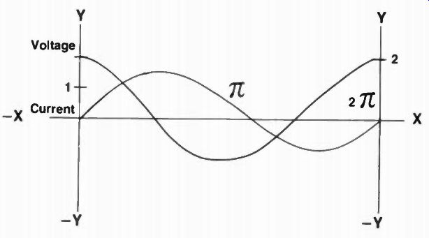
Fig. 8 In a purely inductive circuit, current lags voltage by 90°-or voltage
leads current by 90°.
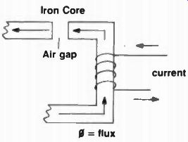
Fig. 10 A magnetic circuit, complete with flux, external windings and current,
and air gap.
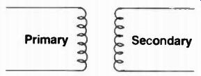
Fig. 9 Two coils, if wound correctly and spaced properly, form a very useful
transformer.
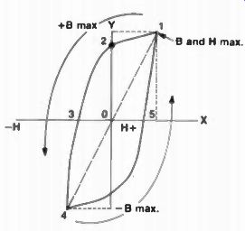
Fig. 11 A typical hysteresis loop.
Sawtooth or ramp waveforms
(Figure 3D) are next and when combined with rectangular pulses they form a trapezoid. Unlike pulse and square waves, sawtooth waveforms are made up of a fundamental (original frequency) and both odd and even (2,3,4,5) harmonics. They are used as deflection currents in large inductances such as TV yokes and a ramp as an internal means of deflection in a sweep generator. Any sync system can find use for a sawtooth when the rise times are quite slow and the fall times not especially abrupt. This is sort of a lazy waveform, but it can produce considerable driving power and may be made extremely linear (where voltage and current are proportional). The trapezoid, shown next to the sawtooth in 3E, is also useful in deflection driving systems where the power outputs are vacuum tubes.
Deflection coils with higher impedances have both inductance and resistance, and both a rectangular (for inductance) and sawtooth (for resistance) must be combined to drive such subsystems successfully. In solid state deflection systems with their lower, largely current-driven impedances, a rectangular wave swinging from near dc to some fairly high power supply level is sufficient. Here, coil dc resistance is negligible.
A triangular waveform (Figure 3F) is the final waveshape that will be considered now. The odd harmonics of this waveform begin at 9, then 25, 49, etc., are spaced far apart, and are not periodically regular. However, a triangle of voltage is useful in low frequency situations where harmonic distortion is easily seen, while high frequency oscillations can also be read on both rising and trailing slopes of the waveform. Crossover distortion-around the zero conduction point of push-pull amplifiers-can also be recognized using a triangular wave, as well as high and low frequency rolloff.
Capacitors
You know that dc currents and voltages power electrical circuits while alternating or digital energy supplies information, the components that have so much to do with these procedures need intensive explanation. For if you know precisely what capacitors (and inductors) do in electronics, much of the remainder is easy. Usually, the inductor is selected initially for explanation because its operations are somewhat easier to follow. But while your attention is fresh at the beginning of this discussion, let's consider capacitors and capacitance first.
Inductors then may follow as both individual units and in combination with resistors and capacitors, forming complete RLC circuits.
A capacitor is any pair of conductors separated by an insulator called a dielectric ... and the insulator may be polyethylene, mica, ceramic, foil, paper„ or even air, etc.
Capacitance is the charge a capacitor will accept and store until such charge either leaks off or the capacitor is discharged. A capacitor has a value of 1 farad when 1 volt/sec. produces a current of 1 ampere. Its charge 0 in coulombs (6.28 x 10¹⁸ electrons) is proportional to its capacitance and the voltage applied across it.
Q = CE, C = Q/E, E = Q/C
where C is capacitance in farads, and E is the applied voltage. One pF (microfarad) is 10^4 farad, and one pF (picofarad) is 10^- 1 2 farad. The term mF stands for (10^-3) millifarads; we now use only the symbol "u" (mu) for micro and ppF is now pF. Energy stored in the charge across any capacitor amounts to W (joules in watt-seconds) and the following equations:
W = 1/2 (QE), Q^2/ 2C, or 1/2 (CE^2)
All are derived from the original Q = CE identity in the paragraph above.
Any parallel plate capacitor and its capacitance may be computed in inches by another equation: C = AK/4.45g where A is the area of one plate, K is the dielectric constant (found in certain tables; 1 for air), and g is the measurement (in inches) between plates.
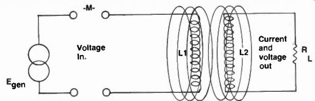
Fig. 12 Two coils in proximity develop mutual inductance, M.
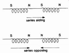
Fig. 13 Series aiding and bucking coils are used for a variety of purposes.
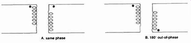
Fig. 14 A phase shift of 0° or 180° induced by different winding starts.
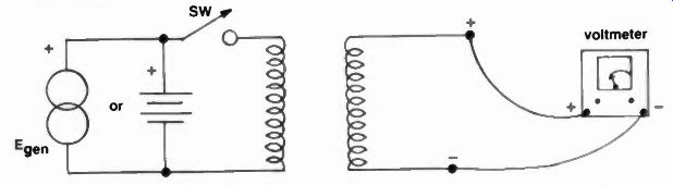
Fig. 15 An experiment to determine transformer polarity.
A capacitor is a memory retention element that accepts and stores a charge until, by some, means it is discharged. The plates of any capacitor are the storage shelves for charges of electrons and the potential between plates across the dielectric is called an electrostatic field. The charge on any capacitor will be determined by the potential applied and the size, or surface area, of the two plates and the dielectric. An expensive, well-constructed capacitor may hold its charge almost indefinitely, but a cheap one, or one of very large value, will permit its charge to leak off in proportion to its size, dielectric, and quality. A resistor in series with the capacitor (Figure 4) may provide a timed period of charge and discharge that can become valuable in waveshaping, determining tube and transistor amplifier frequency characteristics, and audio sound compensation.
Capacitors are used frequently in both dc and ac circuits, where their behavior is often quite different because of steady state and the rising and falling levels of signal generation.
But in both instances, the capacitor is charged and discharged and will react accordingly to surrounding circuit components and the charging source.
Also, its use in both types of circuits differ and therefore, logically, so do its characteristics. In dc power circuits, for instance, large capacitances are needed to filter ripple, and therefore these have internal materials of aluminum, tantalum, etc., while high frequency ac coupling capacitors may be ceramic, mica, polyethylene, or any other similar high quality dielectric.
Capacitors also have both ac and dc potential ratings that many seem either not to understand or to ignore, but these ratings should be considered before particular capacitors are used in certain circuits.
A 400V dc-rated capacitor, for instance, might well operate in a 600V ac circuit, but suffer a breakdown if the ac-dc voltage applied is reversed.
In another instance, a large, somewhat leaky capacitor might be used as a bypass to remove the degenerative effect of an emitter resistor. But the leakage might also shunt the emitter resistor, negating its self-bias, so that circuit parameters would immediately be upset.
Charge & discharge
When any capacitor is charged to store electrical energy, there must be voltage applied to its plates. Figure 5 shows a condition where either a battery or voltage generator is in position to charge a capacitor to its partial or complete potential, depending on the time allotted. With the switch open, of course, no voltage can get to the capacitor, and neither capacitor plate is charged. When the switch closes, however, electrons flow from the battery's negative terminal to the nearer capacitor plate, delivering a negative (an excess of electrons) charge. When this occurs, all electrons on the capacitor's positive terminal are attracted to the battery's positive plate, causing an absence of electrons (holes in a semiconductor), resulting in (a less negative) positive potential. And, although there is current flow to and from the plates of the capacitor, no current flows through it because the dielectric (insulator) between its plates prevents current passage.
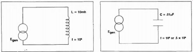
Fig. 16 Coils have ac reactance, depending on frequency.
Fig. 17 Capacitors have reactance inversely proportional to frequency.
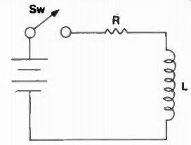
Fig. 18 A coil in a dc circuit charges and discharges exponentially just like
a capacitor.
Nonetheless, the charge and discharge cycle makes it appear as though it does and in practical electronics we say capacitors couple one circuit to another, implying continuous current flow. There is now a voltage across this capacitor that reaches 63 percent of its fully charged state in a certain time. This time is the product of its internal or external resistance in ohms times its capacitance in farads and equals the elapsed time in t seconds: t = RC And this is known as the time constant of a capacitor. Interestingly enough, since current and voltage across any capacitor vary inversely, during the 63-percent charge time, the current is decreasing by 37 percent. Since capacitors charge, they must also discharge, and the same rules apply here, except the RC time constant begins at, say, 100 percent charge and reduces to zero. So as shown in Figure 6, the charge part of the time constant is exponential, as is the discharge portion. In five time constants, the capacitor is fully charged and current stops flowing. As you see, current and voltage across any capacitor are precisely the inverse of one another: when current is maximum there is little or no voltage, and when current is minimum there is maximum voltage. So go back to Figure 1 and remember that in a capacitor, current leads the voltage since, during charge time, a voltage is built up across the capacitor that actually bucks the battery voltage.
This voltage may be calculated from the equation:
e = E(1- eta ^-t/RC)
where e equals the base of natural logarithms (2.718) t equals charge time in seconds E is the battery voltage r amounts to resistance in ohms C is the capacitance in farads Suppose, for instance, you had a 0.01 uf capacitor you were going to charge in 3 microseconds, a battery voltage of 20V, and a series resistance of 100 ohms. The numbers in the equation would now look like this:
e = 20(1-2.718-3 x 10.6/ 10 2 x 0.01 x 10.6)
e = 20(1-2.718-3 x 10⁴/ 104)
e = 20(1-2.718-3) or E = 20(1-e3).
So natural log E(2.718) to the negative 3 can be looked up in the Ex tables, or you can find the log of 1/3 x log 2.718.
Either way, e = 20(1-0.0498) = 20 x .9502 = 19V, and the capacitor is so charged. As the capacitor charges, it may also be discharged, and here we return to current. If the capacitor is fully charged, its discharge current will amount to:
i = -E/Re ^-tRC, simply an Ohm's law E
= IR
equation with the natural log and time constants added along with time.
Don't forget, you are still learning the dc functions of a capacitor! The ac portion is yet to come... With no resistance in the circuit, the capacitor may instantly charge with a current surge; and the smaller the value of resistance, the shorter time the capacitor takes to fully charge.
Inversely, the larger the resistance the greater the charge time because of smaller current flow. So in switch operated circuits, for instance, the smaller the capacitance and resistance, the shorter the charge time until current ceases to flow and the voltage across the capacitor is equal to the battery voltage.
The time constant curve in Figure 6 is also as useful as it is decorative.
For instance, a series resistor of 1,000 ohms and a 0.015 µF capacitor, could have what voltages and currents in 22 microseconds? If the 0 to 100 vertical scale represents ac and dc currents voltages, and the 0 to 5 horizontal scale is in classic time constants, the equations would amount to this: T = RC = 103 x 0.015 x 10-6 = 15 µsec TC = 22/15 = 1.47 So the universal curve reads 1.47 time constants on A, the voltage at E = 77%, and current B (inversely) I = 23% let E = millivolts or microvolts, too, if you like, while I can be amps, milliamperes, or microamperes. The percentages you read out can apply t anything, as long as you stick to equivalent values of volts and currents, or even apples and oranges-if they can charge and discharge with some numerical resistance. Just remember that volts and amps vary inversely as they build or disperse energy, and the combination of the two on a 0 to 100 percent scale must always add up to 100. At this point in this discussion we have a choice-continue on with capacitors in ac circuits, or introduce inductors, carry them through dc and simple ac circuits, and then combine inductors and capacitors in interactive ac circuits. The latter seems the better choice since capacitors and inductors are both reactances in ac circuits and their dual operations can best be explained together. So we'll now move on to simple inductors.
Inductors
An inductor can be any small or large coil of wire that produces an electro magnetic field when current passes through it. The famous left hand rule in Figure 7 shows that when your left hand grasps such a coil with the thumb extended, both the direction of electron flow is established as well as the path (pointing of the fingers) of the surrounding magnetic field. A compass held near the conductor will point north just as your thumb does and verify both magnetic and current direction. Inductance is determined by the number of turns of wire, type of core (many types besides air), turns spacing and method of core winding, diameter of the coil, and the ratio of diameter to coil length. The greater the diameter of a coil, the larger its inductance.
As current increases through any coil, the magnetic flux about the individual turns expands and cuts adjacent turns. The effect is to induce current to flow in the opposite direction, building up a voltage (Lenz's law) that opposes the original current flow. Translated, this means that (Figure 8) current in an inductor lags the voltage by 90 degrees. Also, a decrease in current flow through an inductor induces another voltage that opposes this second change of current. As you will see later, an inductor is very useful as a choke in ac filter circuits to oppose ripple, and can be counted on to produce a large spike of reactive voltage whenever its electromagnetic field is suddenly collapsed and/or its current reversed.
Two coils placed near one another can form a transformer (Figure 9) another useful device whose magnetic flux makes possible excellent circuit coupling without dc voltage interaction and also convenient impedance matching.
Cores and reactance
The core of a coil or transformer is actually a magnetic circuit that passes flux, and this flux depends on MMF-magnetomotive force (equivalent of electrical EMF electromotive force) and also the reluctance (analogous to electrical resistance) internally contained. The equation for such magnetic reaction is very similar to E = IR Ohm's law except for the terminology: F = OR; 0 = FIR; R = F/0 ... a group of similar equalities, where F is the magnetomotive force in gilberts; 0 (Phi) is the total number of lines of flux (Maxwells); and R is the reluctance of 1 cm3 of air (or a vacuum). Such reluctance may be added in series or parallel, just like resistances. In Figure 10 is an illustration of such a magnetic circuit having all the elements of flux, external current (though windings), the iron core, and an air gap. The magnetomotive force F then can have a new relationship: F = 4 /n 10 (NI) = 1.257 NI where N is the number of wire turns, and I is the current in amperes. We may now also speak of the number of lines/in^2 or lines/cm2^ in terms of flux density, B. so that: B = 0/A; A = 0/B; or 0 = BA. "A" being the cross sectional iron core in in2 or cm^2 through which the magnetic path passes.
The magnetizing force H is now identified as the magnetomotive force F in gilberts/cm. divided by the length of the path in centimeters: H = F/L Coil inductance is also proportional to its core permeability, and permeability p is flux density in gauss B divided by the magnetizing force H in oersteds: p = B/H, Flux, of course, is equivalent to conductivity in electrical circuits, but varies with generated flux.
Skin effect is confined to ac systems (not dc), and is a term used to describe the contraction of flux at the center of a coil (or wire) and its expansion about the perimeter with varying current amplitudes.
Consequently, wire impedance will be greater within the conductor than on its surface, so ac, naturally, will take the path of least resistance and follow the outer coil path. This effect is especially noticeable at high energy rates because inductive reactance is always proportional to frequency.
Radiation loss is another high frequency consideration that can become serious at upper megahertz and gigahertz frequencies.
Eddy current losses occur when coils are subject to a varying magnetic field-and since each conductor is cut by lines of flux, differences in potential result in a number of auxiliary currents being developed that serve no useful purpose. Unfortunately, they produce both heating and additional resistance which must be made up by added energy applied to the inductor.
Dc resistance of any coil is resistance measured with an ohmmeter and results from the type of material (copper, aluminum), length and diameter, and the effects of temperature.
A coil has an inductance of 1 henry when a change of 1 ampere/sec. of current produces a back emf (electromotive force) of 1 volt.
Hysteresis
For some strange reason, hysteresis arises as the biggest goblin in simple magnetics. Once and for all, it is just a power loss in magnetic material; and this power loss is illustrated by the peanut-shaped curve in Figure 11.
Very simply put, flux density B and magnetizing force H increase from 0 to positive peak 1 then decrease, with hysteresis following the curved path from 1 to 3, passing zero magnetizing force point 2, called the remanent flux density, and reaching 3, where the residual magnetism amounts to zero.
The magnetizing force goes negative, to point 4-equivalent to point 1, but 1/2 cycle later-and then begins its increase toward maximum value, with the hysteresis curve continuing from 4 to 5 and then back to 1. The dotted line between points 1 and 4 is the B (flux density), H (magnetizing force) route and is the normal magnetizing direction.
Mutual inductance
When two coils are placed together so their magnetic fields are joined, a flux common to both loops is generated called mutual inductance (Figure 12). This mutual inductance M depends on the coils relative positions (to one another), their permeability (II = BM), and the inductance of each coil. If two coils are coupled either tightly or loosely, they develop a coefficient of coupling called k, which is usually about 0.5 or less (except for power) and is a constant.
k = M L2 with M standing for mutal inductance and L1 and L2 the primary and secondary of the two coils which now amounts to a transformer. Of course, if you know k, and the inductances of Li and L2, mutual inductance is reasonably easy to find--just a little algebra:
k 2 = M2/L1 L2, then M2 = k 2L,L2 or M
= k\v/ LiL2 and then L1, for instance could be found as easily as L2: L1 = M2/k2L2 etc., if the other values are known. similarly, U = m2/k2 u. The maximum value of k by the way, is 1 ... so that when flux from one coil cuts all turns of the other, unity coupling has been achieved, and this is when k equals 1.
Aiding and bucking
Coils in working circuits are often tapped for impedance matching, separated for filtering and transformer action, placed in series and parallel for specific resonances, and in shunt (across one another) to construct transmission lines, and produce certain phase shifts. In a series aiding situation, (Figure 13) the north and south poles of each coil are connected to one another, and therefore flux produced in each coil combines with the other so both together produce an inductance total of:
Lt = L1 + L2 + 2L_mutual
But in the windings of these coils are series bucking, the total inductance is then less than either coil, and flux lines are consequently reduced. The total of the two still add, but the mutual inductance of the coils is now subtractive, so the equation looks like this: Lt = L1 + L2 - 2L_mutual
Of course such coils may be placed in parallel for both series adding and bucking, and the equations would amount to the same as series resistors except, of course, the addition of L. to each term. For instance aiding amounts to: 1/L, = 1/L I + L. + 1/U + L. while opposing is: 1/L, = + 1/ U-L. Such coils, naturally, can also be separated and used in different ways to change phase in transformers, and can be identified schematically by placement of the dots. If the dots are as shown in Figure C, 14A, the coils and flux are aiding, and there is no phase change but in Figure 14B, the voltages of the unloaded secondary are 180 degrees out of phase with the primary and, therefore, the output is inverse. Usually, most transformers are wound so that the polarities of their primaries and secondaries differ, and if dots are not shown on the transformer schematic, you may assume a phase difference of 11 or 180 degrees. If there is any doubt as to polarities, a signal generator or battery can be inserted in the primary half of a transformer and a dc voltmeter across the secondary Figure 15. If, when the switch is closed-and this has to be the case for instantaneous voltage from the battery-the meter kicks positive, the two coils are wound from the same starting point and the resulting voltage is in phase. If the voltmeter pegs, or goes upscale only when its polarity is reversed, then the secondary windings are in opposition and there is a 180 degree phase change. Switch SW is needed because steady state batteries cannot produce a coil interchange of flux after initial turn on; only alternating voltages can.
Reactance and Time Constants
The temptation at this point is continue immediately with transformers, and leave other coil knowledge for the combined circuits, but this could become confusing, especially since capacitive reactance has already been treated separately.
So we'll work through the remaining inductive characteristics before considering the subject of real transformers, rather than simply the set of unleaded, air-core coils.
Inductive reactance, therefore, is the electromotive force (emf) opposition that builds up within a coil to oppose the flow of alternating current. To sound slightly sophisticated, it amounts to: e = L di/dt or LAi/At where L is the inductance and di or Ai and dt or At mean the rate change of current with respect to time.
Calculated with inductance, they produce the value of the counter-emf developed across the inductance. The triangular symbol, of course, is called delta, and represents a larger increment than the differential di/dt.
The instantaneous value (in ac) of this current is: i = I m sin wt (where w = 2 n f, or 6.28 x frequency)
The instantaneous value (in ac) of the voltage is: e = wLIm cos wt = maximum current at that instant)
So, by now, you can begin to pull together the sine alternation and the cosine alternation, and mentally visualize the current-because of the resulting counter emf-actually lagging the voltage in a purely inductive circuit by 90 degrees. And, because of the counter emf, current is choked and physically reduced in magnitude. The opposition to this current flow at differing frequencies is called inductive reactance and results in the equation: X, + w L or 2 pi fL since w = 2 pi In Figure 16 for instance, if a generator is pumping in a sinewave at a frequency of 1MHz, and the coil value is 10 millihenrys (mH), the inductive reactance at that frequency would be: X, = 6.28 x 106 x 10 x 10^-3 = 62.8 x 10^3 or 62,800 ohms at 500KHz -half the frequency-the reactance of this coil would decrease to: X, = 6.28 x .5 x 10^6 x 10 x 10^-3 or 31,400 ohms, exactly half.
The capacitive equation (Figure 17) is: X,. = 1/2 fC = 1/6.28 x 10^6 x 0.01 x 10^6 = 1/.0628 = 15.9 ohms but X, = ½ fC at 500 kHz amounts to X, = 1/6.28 x .5 x 10^6 x 0.01 x 10^-6 = 1/0.314 = 31.9 ohms and this is just about double the reactance as the frequency decreases by half. So we can truthfully say that the reactance of a capacitor changes precisely opposite to that of an inductor with changes in frequency. Such opposing reactions are highly useful in maximum power transfer (impedance matching), filters, waveshaping, and resonant circuits, etc. Now, with inductors and capacitors having different responses under similar circumstances, additional methods are needed to calculate what their reactive impedances and phase angles are going to be as alternating currents and their driving voltages change.
Time constants for the inductor have considerable similarities to those for capacitors, and both can use the same charge-discharge curve (Figure 6). However, an electromotive force is present to oppose current changes, and therefore we think of inductors in terms of current rather than voltage.
Both charge and discharge equations follow the capacitor's rules (Figure 18), except that resistance R is now on the top portion of the exponent with the L below, whereas in the capacitor, both R and C (RC) were below the exponential line and divided into time t. The natural log to the base E continues to be used as does the usual voltage and resistance. So in dc circuits, the equations look like this: i = E/R(1 . e - R") with i in current (amps), tin seconds (after the switch is closed), inductance L in henrys, dc volts in E, and total circuit resistance in R (ohms). Here, time constant T is the time in seconds from the moment the switch is closed until current has risen to 63 percent of its full value and amounts to the equation: T = LJR where L is the inductance in henrys and R the resistance in ohms. An inductance of 15 mH, for instance, might have circuit resistance of 1K ohms. So the time would be: T = 15 x 10^-3/ 10^3 = 15 x 10^6 or 15 microseconds.
If we wanted to know the current through such an inductor with E representing 20V:
i = 20V/10^3 (1-E- R") and -RilL = -1 03 X X 15 x 10-616 x 10.3
i = 20 x 10^-3 (1-c.1)
i = 20 x 10^-3(1 0.3679)
i = 20 x 10^-3(0.6321) = 12.642 milliamperes
That, being the charge circuit, the discharge equation is simply:
i = E/R(s- "L,) and, of course, the calculations are done in exactly the same way except there is no subtraction of the natural log product from 1. Surprisingly, the charge and discharge curves are spoken of as transients, because such an electrical action would be a one time occurrence and not ordinarily repetitions.
To be continued
Brush up on your trigonometry. Next month we'll discuss vectors and get into complex circuits of resistance, capacitance and inductance, things you haven't thought of lately.
(source: Electronic Technician/Dealer)
Also see: Link | --AC Theory and Reactive Networks, Part 2--More About AC