SOME records are cut with a constant-velocity response curve, others with a constant-amplitude curve. Still others--ordinary phono graph records, for instance--employ a combination or modification of these basic methods. What is meant by these two terms? What are the uses and comparative advantages of these methods of cutting? The frequency response of the entire recording system can be judged and measured correctly only when they are thoroughly understood and applied. Curves are meaningless unless the differences between constant amplitude and constant velocity are understood.
Constant Amplitude
First consider the action of the crystal cutter. In a piezo-electric crystal, the amount or amplitude of physical twist or distortion-and therefore the distance the stylus moves-is dependent on the value of voltage, regardless of frequency. In the crystal cutter, it is the groove width or amplitude which is directly controlled by the voltage. If the frequency is high and the voltage to the cutter terminals is kept constant, the amount of stylus travel is just as great as it would be at lower frequencies. If the stylus is to cut as wide a path at 2,000 cycles as it did at 1,000 cycles, it must, of course, travel faster. Stylus velocity, in a crystal, is therefore variable.
If stylus travel is dependent only on input voltage, with velocity changing as necessary to keep inches of travel constant, frequency will not be a factor. This is shown in curve A of Fig. 601. Since the vertical axis denotes amount or amplitude of stylus displacement, the curve will have to be flat if the input voltage is constant. We may then call the response of a perfect crystal cutter a constant-amplitude response.
A perfect crystal pickup has the same characteristic: output voltage depends entirely on amplitude of groove variations, without relation to frequency. Thus both crystal cutter and pickup are constant--amplitude devices, and curve A in Fig. 601 is a constant-amplitude curve. The pickup's response complements that of an ideal crystal cutter. The pickup delivers a constant output voltage when playing a record cut by a constant-amplitude crystal cutter.
Constant Velocity
Now consider the magnetic cutter. Stylus movement is produced by movement of the armature, which, in turn, is produced by reaction of an electromagnetic field with a permanent magnet field (see Section 5). In a motor-which the cutter is-speed or velocity of movement of the coil and its armature is directly dependent upon the magnitude of the impressed voltage. Note that nothing is said about the total amplitude, or distance of the movement. A motor armature will continue to rotate as long as voltage is applied to it. Only the velocity is affected by the voltage.
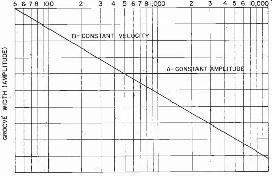
Fig. 601--Outputs of ideal constant-amplitude (A) and constant-velocity
(B) record, reproduced on ideal constant-amplitude pickup.
When we apply d.c. to the armature winding of a magnetic cutter, the stylus moves at a velocity determined by the amount of voltage. It will continue moving--in the same direction--until either the voltage is removed or the armature is physically restrained from moving further by the dampers and pole pieces. When we apply an audio voltage, the reversal of polarity at the end of each alternation limits stylus travel, just as removing the d.c. voltage did.
Fig. 602--a shows a 1,000-cycle sine wave of a certain voltage. If the entire cycle takes 1/1,000 second, then one-half the cycle will take 1/2,000 second and one-fourth the cycle will take 1/4,000 second. At point A (the beginning of the cycle) the voltage is zero. Now look at the cutter in Fig. 602-b. Point A is the normal position of the stylus with zero applied voltage. During the first quarter-cycle AB, voltage will rise to maximum in the positive direction and velocity and direction of movement will be imparted to the stylus. Velocity at any instant depends on the instantaneous magnitude of the voltage, while direction depends on the direction of electron flow in the coil. The velocity at the selected audio voltage is such that in the 1/4,000 second occupied by the first quarter-cycle, the stylus will have time to move from A to B (Fig. 602-b). At the beginning of the second quarter-cycle (point B on the graph), the direction of current flow reverses and the stylus begins to return to its center position A which it reaches just as the instantaneous voltage reaches zero. The same process is repeated, but in the opposite direction, for the second half-cycle.
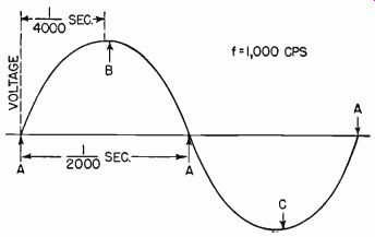
Fig. 602-a--A 1,000-cycle sine wave, showing time relations for 1/4
and 1/2 cycle.
Consider Fig. 603, drawn to the same scale as 602-b. As before, at the given r.m.s. voltage at 1,000 cycles, the stylus moves from A to B and back in the first half-cycle and from A to C and back in the second half. Now let us apply a frequency of 2,000 cycles at the same voltage. During the first quarter-cycle the stylus will travel toward B again, but at 2,000 cycles a quarter-cycle lasts only 1/8,000 second.
The voltage and the velocity of the stylus movement have been kept constant, but the time allowed has been reduced to one-half of its former value. Therefore, the stylus can move only one-half the distance, to point D. During the second half-cycle at 2,000 cycles, the stylus travels in the reverse direction but has only time to reach point E before the polarity reverses. When frequency is doubled, the distance of stylus travel, or stylus displacement, is halved. The armature simply does not have time enough to go as far as it did at 1,000 cycles by the time polarity reverses.
We have simplified this explanation to avoid entanglement in such matters as phase difference in inductive circuits.
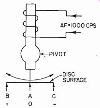
Fig. 602-b-Stylus moves back and forth, through point A, following voltage
changes of Fig. 602-a.
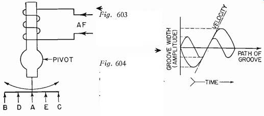
Fig. 603--Stylus amplitude will decrease as frequency is increased.
Fig. 604--To keep slope or velocity constant, amplitude must increase as frequency de creases, and vice versa.
Velocity can be represented by the slope of the wave at its zero point. As Fig. 604 shows, to keep slope or velocity constant, amplitude must increase as frequency decreases, and vice versa. The 2 sinewaves have the same velocity, but their frequency ratio is 1 to 2 and amplitude ratio is 2 to 1.
In an ideal unequalized magnetic cutter, to which constant voltage is applied, stylus displacement or amplitude is inversely proportional to frequency. At any given frequency the stylus cuts a groove with width twice that of an octave above and half that of an octave below. (An octave is the interval between a given frequency and one either half or twice its value.) If frequency rises, stylus movement or amplitude decreases in proportion ; if frequency drops, amplitude increases in proportion. This relationship between frequency and stylus movement is the crux of constant velocity and must be under stood fully. The ratio of groove width at any frequency to groove width at one octave above that frequency is 2 to 1. We can evaluate the groove widths in terms of voltage. A voltage ratio of 2 to 1 is equal to a decibel gain or loss of 6. We can now be exact when speaking of the frequency response of a magnetic cutter: output of the cutter decreases at the rate of 6 db per octave with increasing frequency.
Curve B in Fig. 601 shows this response.
The situation in a magnetic pickup is exactly opposite to that in the cutter. In the pickup, movement of the armature through the magnetic lines of force created by the magnet induces a voltage in the coil.
The velocity of armature movement determines the magnitude of the voltage induced. Velocity depends on two things: the frequency being picked up, and the width of the groove. As frequency goes up, velocity of the pickup needle and armature increases. Increased velocity means increased output. We can also increase armature velocity (without changing frequency) by increasing groove width, for now the needle must travel a greater distance in the same period of time. Thus, pickup output (at any one frequency) increases as groove width is increased.
But the magnetic cutter cuts narrower grooves as frequency is raised.
This of course means lower velocity for the pickup armature. The effects of raising frequency and decreasing groove width (or vice versa) are exactly opposite and nullify each other. The result : pickup armature maintains constant velocity (and constant output) at all frequencies when playing a record cut with an ideal magnetic cutter.
In this discussion, the input voltage to the cutter terminals was assumed to be constant in value throughout. The frequency response of the magnetic cutter is the result of the fact that a constant applied voltage will produce a constant velocity of stylus movement. The response of magnetic pickups-exactly opposite to that of magnetic cutters-occurs because constant velocity of needle movement will produce constant output voltage. Any similar cutter or pickup curves are known as constant-velocity curves ; and the devices which produce them are known as constant-velocity devices.
To summarize briefly the differences between the 2 types of cutter response: in constant-velocity cuts, groove width decreases (6 db per octave) as frequency goes up; while in constant-amplitude cuts, groove width remains the same for all frequencies. Stylus displacement versus frequency curve for each type of response must be memorized Modified Constant Velocity The patterns in Fig. 605 are enlarged drawings of record grooves showing variations in the width of the groove at various frequencies.
Pattern 1 shows a perfect constant-velocity cut, the same as curve B in Fig. 601. Notice that the groove variations are very large at the low-frequency end and become progressively smaller as the frequency rises.
The groove width at 100 cycles is about 100 times as great as at 10,000 cycles.
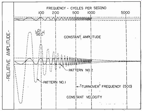
Fig. 605--Wave patterns for constant-amplitude, constant-velocity (pattern
1) and modified constant-velocity (pattern 2) recording.
In practical recording, the distance of adjacent grooves from each other limits maximum groove width at low frequencies. If the stylus is allowed too much travel, it will cut into the next groove and ruin the recording. By limiting the audio signal level fed to the cutter, we can prevent this overcutting of adjacent grooves. However, groove width will be so slight at the high-frequency end of the audio range that the groove variations will be comparable to the random surface irregularities of the disc which produce scratch and surface noise. The noise will bury the signal. Under these conditions, the; ratio of maxi--mum groove width (at low frequency) to minimum groove width (at high frequency) is too great to be practicable.
There are 2 solutions to this problem. The first is the use of constant-amplitude recording. This is shown graphically in curve A of Fig. 601 and pictorially in Fig. 605. The groove variations are just the same at the low end as at the high end. Records can be and actually are cut in this manner, without any modification. Crystal cutters are used, and the records are played back on crystal pickups.
Phonograph records and most professional discs are not made constant-amplitude, however desirable it might seem. Phonographs and professional playback systems are still geared to the older type of recording, constant velocity, and manufacturers of records are still chary of changing their discs. The method of reducing the minimum-maximum groove width ratio in general use is to modify both types of curve and use a combination of them. The result is known as modified constant velocity.
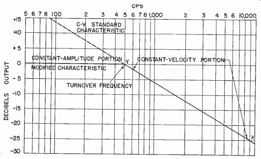
Fig. 606--Commercial modified cons ant-velocity record response, when
pickup has constant-amplitude characteristic. Turnover is arbitrarily
placed at 500 cps.
Observe pattern 2 in Fig. 605. From 500 cycles upward, groove width decreases as frequency rises, just as in the perfect constant-velocity curve. But from 500 cycles downward, groove width remains constant. From the lowest frequency up to 500 cycles the pattern is the same as that for constant amplitude. The ratio between maximum and minimum groove widths is much reduced. If low-frequency stylus travel is increased to the allowable limit, high-frequency groove width will also be increased to a usable value.
This modified-constant-velocity curve is shown graphically in Fig. 606. This graph is plotted just as Fig. 60 ; the vertical axis may be thought of as stylus displacement or groove width. The curve is in 2 distinct parts : constant amplitude up to 500 cycles, and constant velocity beyond that. Turnover frequency, the point at which the change in type of response takes place, is usually 500 cycles in U.S. records, and has been 300 cycles in most European recordings. In some broadcast transcriptions it is 1,000 cycles. Since there is very little standardization, the turnover frequency may be any frequency arbitrarily chosen by the recordist. For discussion purposes, we will stick to 500 cycles.
Response Graph Conventions
The graphs we have shown so far have been based on groove width versus frequency. However, these are not the graphs commonly used or published by the industry.
Since the constant-velocity characteristic is the principal basis for recording today, it has been taken as the standard for comparison. In other words, specific cutters, pickups, and records are compared to the standard constant-velocity characteristic, shown in Fig. 601. Curves published do not actually show a picture of stylus displacement ; they show the difference between the device or record being discussed and the standard characteristic.
To illustrate this point, compare Figs. 606 and 607. They both represent identical responses, the modified-constant-velocity response described above. However, Fig. 607 is drawn on a constant-velocity basis, which means that it is not a picture of anything real ; it is only a comparison with the standard, ideal constant-velocity response.
The upper portion of the modified curve (between points X and Y of Fig. 606) corresponds exactly to the standard constant-velocity characteristic. Since the actual modified characteristic--shown in Fig. 606--agrees (from 500 cycles upward) with the standard, there is no difference between them. Therefore, when drawing a curve of comparison, all points from 500 cycles upward will have to be on the zero line, showing zero difference. See Fig. 607.
Below 500 cycles, however, the modified characteristic does show a departure from the standard. At 250 cycles, for instance, Fig. 606 is 6 db below the standard. Therefore, the 250-cycle point in Fig. 607 must be at-6 db.
Fig. 607 is the usual curve used in recording literature, and is a comparison with the ideal constant-velocity groove-width response curve. If, for instance, the graph shows response at 100 cycles to be at-14 db, it means, not that groove width has been reduced, but that actual pickup output voltage is 14 db less than would be obtained from a perfect constant-velocity record.
This curve, is, in fact, a graph of the output voltage obtained from a perfect magnetic pickup. We have seen why the low-frequency section is purposely reduced. If we use a magnetic pickup to play these records, we must insert an equalizer to boost the low frequencies, as Fig. 607 indicates.
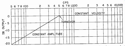
Fig. 607--Modified constant-velocity record response when played on
perfect uncompensated constant-velocity pickup. This is the standard "velocity
basis" type of curve, a comparison with the theoretical curve B
of Fig. 601.
The modified curves in use by different manufacturers of records are not usually identical. While Fig. 607 illustrates the modified type of response, there are many variations of this. The high end may be increased, and other turnover frequencies may be used. They may, however, all be plotted just as Fig. 607 was plotted, as comparisons with the standard, or, speaking in a more practical manner, in terms of the output voltage obtained from a perfect unequalized magnetic pickup.
The modified characteristic is built into most commercial magnetic cutters by means of mechanical adjustments and rubber dampers. It is usually unnecessary to provide for the low-frequency drop by equalizing the recording amplifier.
When speaking of records which are cut completely constant amplitude, these curves of comparison with a constant-velocity standard are not used. The literature on constant-amplitude work shows crystal cutter curves merely as straight lines (or variations of that ideal).
Fig. 608 might represent the response of a perfect crystal cutter. This curve does not have the same significance as those usually seen for constant-velocity devices. Here, it means that stylus displacement of the cutter is uniform over the range, and that an ideal crystal pickup will produce output as shown. Such curves are always accompanied by explanations unless they represent performance of crystal devices, in which case it can be assumed that they are curves of actual stylus displacement.
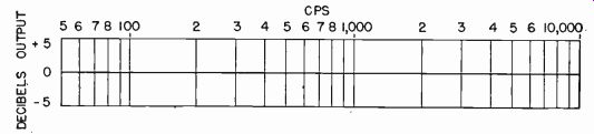
Fig. 608--Perfect crystal cutter response. This is NOT a comparison with
the standard C-V curve.
Summary
The material in this Section requires careful, thoughtful reading, but can be understood by the average radioman. Let us briefly summarize the points we have covered :
1. In the crystal cutter, stylus displacement is the same no matter what the frequency. Crystal pickups are identical.
Curves showing crystal response show actual stylus displacement. The crystal characteristic is constant amplitude.
2. In the magnetic cutter, stylus displacement decreases as frequency rises, and vice versa, but velocity remains constant. In the magnetic pickup; velocity determines output, and the resultant output is flat. The magnetic characteristic is constant velocity.
3. In practice a modified-constant-velocity characteristic is used, consisting of constant amplitude up to a turnover frequency between 300 and 1,000 cycles (usually 500 cycles in the U.S.A.) and constant velocity thereafter.
4. Conventional curves show, not actual stylus displacement, but output of a record as played on a perfect magnetic pickup. A flat cutter and pickup will therefore show output as a flat line.
Constant-amplitude recording has advantages. It is linear and there is no turnover frequency to worry about. The high-frequency groove width is made just as large as low-frequency width, and the signal-to-noise ratio is very good as a result. The record may be played back on a high-quality crystal pickup without any equalization. Results, even on a cheap crystal pickup, will usually be better than obtained from the usual records.
Crystal cutters are quite versatile. With very simple variations in the method of connection to the recording amplifier, many different recording curves, including the modified-constant-velocity characteristic used on phonograph records and shown in Figs. 606 and 607, may be obtained. The methods of varying crystal cutter frequency response are shown in detail in Section 11.
Remember that curves of crystal and magnetic devices cannot be mixed. If, for instance, the curve of Fig. 608 represented a crystal pickup and that of Fig. 607 a magnetic cutter, we would expect the output to be flat above 500 cycles. If it is remembered that Fig. 607 is plotted on the usual velocity basis while Fig. 608 is on an amplitude basis, representing stylus displacement, it will be clear that one or the other will have to be converted to the opposite basis before a true picture of output can be had.