WE will first deal with amplifier measurements because these are necessary to establish the basis for tests on equipment that we will come to later in the guide. We have to rely on calibrated basic amplifiers with a flat frequency response and linear performance (or known deviation), before we can interpret other measurements.
Frequency response
The important thing in making a frequency response check is to eliminate possible sources of error due to measuring equipment. The classic way of determining response uses some kind of meter to indicate voltage levels at various frequencies. Most voltage measuring instruments are subject to a 1% or 2% deviation in calibration as well as a response that will vary at different frequencies. So, if this kind of instrument is used for precision measurement of frequency response, we must devise a means of eliminating its own characteristic variations.
The common method is to use a calibrated attenuator. (See Fig. 215 in Section 2.) The simplest is one with three decade steps: one in 10-db per position, the next in 1-db units and a final decade of 0.1-db units. This enables the attenuation to be read to within 0.1 db over a range up to 100 db. An input voltage equal to the desired output voltage is applied to the input terminals of the attenuator. The amplifier output is loaded with the required nominal dummy load resistance and a dpdt switch is connected between the input to the attenuator and the output from the amplifier, so the vtvm can be switched between these two positions (Fig. 401).

Fig. 401. Basic arrangement for taking the frequency response measurement
of an amplifier.
The procedure consists of setting the oscillator input to the predetermined voltage on the vtvm. It may be half the maximum output voltage of the amplifier. Maximum attenuation is inserted.
Then the switch is thrown to measure the output, and the attenuator is adjusted until exactly the same reading is obtained. The gain of the amplifier must then be equal to the loss in the attenuator. This operation is repeated at a number of frequencies from the lowest to the highest required and the result is plotted in the form of a frequency response.
The frequency response of an amplifier is measured, at a variety of levels, representing from somewhere in the region of one-tenth of maximum output up to full output. In the region of maximum output monitor the output voltage with a scope to be sure the waveform remains reasonably sinusoidal. If appreciable distortion occurs, the vtvm will introduce a waveform error and we will have no means of knowing precisely when the input voltage, which is sinusoidal, is equal to the output voltage, which is not. So a frequency response taken at a level where some frequencies are distorted becomes invalidated because of the output waveform distortion.
Using this method of measuring frequency response, some manufacturers have produced an instrument called a "gain set." It consists of a vtvm, an input-to-output switch and the calibrated attenuator, all in one instrument.
If the gain set has been well built, there is no reason why it should not perform as well as the separate components. However, the author's experience has been that most available gain sets show some form of deficiency. Either the attenuator is off calibration or the vtvm does not work correctly, etc. There is no reason why such faults should develop more readily in a packaged unit, than in a set of separate components, but the problem does exist.
While this measurement technique may be academically more accurate (once you have checked the equipment) a method that is gaining acceptance because of its more informative nature is the input-output comparator used with a scope. If you already have the calibrated attenuator, this can still be used; otherwise an uncalibrated attenuator will serve just as well. As the scope does not rely on rectifying the signal it displays, but gives a linear deflection of the spot for input voltage, and the scope amplifiers can be calibrated to give as near flat frequency response as desired, the scope method of measuring can be made independent of frequency errors characteristic of the vtvm.

Fig. 402. The audio oscillator-comparator method of measuring frequency response
and other details of amplifier performance.
To use this method connect the oscillator output directly to both scope inputs, and adjust the scope's vertical and horizontal gain controls to get a line at 45° that almost fills the screen. Sweep up and down in frequency over the range to be used in measurements, to see whether the line opens out into an ellipse or changes slope. If it does, careful calibration of the gain and phase differentials involved must be made, on each range of the scope amplification, by the method outlined in the section on basic measurements. This has to be applied as a correction factor to all measurements, carefully working out whether the adjustment is added or subtracted. A response that rises with increasing frequency is accompanied by phase advance, while one that falls corresponds with phase delay.
Most precision scopes will not need appreciable correction of this nature. To make the actual measurements, connect the input point that went to point A of the switched vtvm (Fig. 401) to the horizontal input, and the output of the equipment under test to the vertical input (see Fig. 402). Having set the attenuation and oscillator levels to get the required operating condition at 1,000 cycles, adjust the scope amplifiers to obtain a 45° trace of convenient length. Now the frequency can be swept, and the effect ob served without resetting the scope gain controls.

Fig. 403. Display pattern sequence (left-hand pattern is mid-band, others
progressively higher or lower) showing how to identify a characteristic where
-3db and a 90° phase shift coincide.
The advantage of this method is that it compares, not only the relative magnitudes of input and output voltages, but also indicates the transfer phase of the system. This can be useful in deter mining whether the stability characteristic of the amplifier is satisfactory. A good rule for this is to check the frequency response to the point where the phase transfer angle from input to output is 90°. The condition for maximum flatness in the pass range which corresponds with the ideal stability margin occurs with an attenuation of 3 db (at the 90° point) compared with mid-range.
This is quite easy to observe on the pattern. As the oscillator frequency is varied from mid-range (1,000 cycles), watch for the points where the ellipse lies in a horizontal plane rather than its usual sloping aspect. By means of the oscillator output control adjust the length of the ellipse to the same horizontal length as the original sloping line. Then its height will be about 0.7 of the mid range height of the sloping line (Fig. 403) if the loss is 3 db at this point. For practical purposes, if the ellipse becomes a circle at the 90° point, and if the peak between mid-range and this point is not more than 1 or 2 db, the amplifier will give acceptable performance.
These measurements should be made using a resistive load. As a further check, a similar run may be made into a speaker or other reactive load, when more latitude in the precision of the measurement can be tolerated. For reasonable performance the peak at 90° should never exceed 6 db (twice the original height of the trace).
In addition to measuring the frequency response of the amplifier at different levels with the gain control wide open, check the amplifier with the gain control in other positions. The position in which it is likely to make the greatest difference in the frequency response is at precisely 6 db below the wide open position. To find this point turn down the gain control until the output voltage is just half its previous value. Then recheck the frequency response by either of the methods just described to see what effect the gain control has.
Gain

Fig. 404. For 600-ohm amplifier input, this provides the termination for the
attenuator (a), but for a high-impedance input (b) an external terminating
resistor must be used.
The same setup for measuring frequency response can be used for checking either gain or sensitivity. Gain is usually output divided by input. This may be given in terms of voltage or power, specified, respectively, as voltage gain or power gain. For example: if the attenuator reading is 46 db, (which corresponds to a ratio of 200) the voltage gain is 46 db and the input sensitivity the full output voltage (say 15 volts) divided by 200 (75 my).
Power gain is obtained simply by making a transformation to account for the change in impedance between input and output.
The output is usually a speaker impedance of 4, 8 or 16 ohms (or it may be 600 ohms) while the input impedance with tube type amplifiers is usually high or it may be transformer--matched to a 600-ohm line.
Where input and output impedances are both 600 ohms, the voltage gain is precisely the same as the power gain. Under this condition it is important that the attenuator be designed for 600-ohm operation. If the input impedance is high, a 600-ohm attenuator will also be used, but it will require a terminating resistance of 600 ohms because the amplifier does not provide this.
This distinction is illustrated in Fig. 404.
Where the input is a high impedance, it is normal to specify a voltage gain for the amplifier or to specify the sensitivity in terms of output power for a given input voltage. The input voltage can be calculated from the voltage used for measurement and the amount of attenuation used in the gain set. With the comparator method, the attenuation between the takeoff point for the scope and the actual input to the amplifier must be calibrated and the voltage at the scope takeoff point measured so that the actual input voltage to the amplifier can be calculated.
If the input is 600 ohms and the output some other value, a correction factor must be used to calculate the gain. This is obtained by adding 10 times the logarithm of the impedance stepdown ratio. If the input impedance is 600 ohms and the output impedance 16 ohms, then the impedance stepdown ratio is 37.5 to 1. This means the power gain will be 15.75 db more than the voltage gain (10 x log 37.5/1 = 15.75 db) . If the voltage gain is 26 db (which will mean, for example, that 0.25-volt input will produce a 5-volt output), the power gain of this particular amplifier would be 26 + 15.75 = 41.75 db.
Another term often encountered is the "insertion gain" of an amplifier or system. This, unfortunately, has two definitions. It is best, of course, to use the modern one, but keep in mind that past literature may refer to either.
The modern definition states simply that insertion gain is the increase in power transfer produced by connecting the amplifier between the source and load. The older definition states that the comparison should be between the transfer when the amplifier is connected and when an ideal matching transformer is connected in its place.
Suppose the input impedance is 600 ohms and the output 16 ohms, and that 1-volt input at the amplifier terminals gives an output across a 16-ohm load of 10 volts. This is a voltage gain of 20 db, or a power gain of 20 + 15.75 = 35.75 db. Now we are faced with the question-how much power would be delivered to the 16-ohm load by direct connection? There are various answers to this question. Assume that the source resistance is also 600 ohms, as it will be with the gain-set method. Then 1 volt at the amplifier input terminals is equivalent to 2 volts applied through a series resistor of 600 ohms, assuming the amplifier presents an input load of 600 ohms. In this case, using the modern definition, feeding 2 volts through 600 ohms into the 16-ohm load will deliver:
16 E2 2 X = .052 volt or 0.17 milliwatt (watts = 16 600 R)
The 10 volts across 16 ohms when the amplifier is connected is an output of 6.25 watts. So the insertion gain, by modern definition, is the ratio between 0.17 mw and 6.25 watts, or 45.7 db.
Following through with the same example, for the old definition we should use a theoretical ideal transformer to convert the 16-ohm load to 600 ohms. The hypothetical substitution will still produce 1 volt across the 600-ohm primary in place of the amplifier's 10 volts across 16 ohms, an insertion gain that represents the same increase in power as our definition of power gain, 35.75 db.
These figures are on the assumption that the source resistance, as well as amplifier input resistance, is 600 ohms. Other extreme possibilities for this example are either that the source resistance is much lower than 600 ohms-zero in the ultimate, or that the input load of the amplifier is much higher than its nominal 600 ohms-open circuit in the ultimate. Either way, the input voltage will be 1, whether or not the amplifier is connected.
In the first case, using the new definition, connecting the 16-ohm load directly to the input source will still produce the 1 volt delivered to the amplifier input (in theory, at least), instead of the 10 volt output the amplifier gives. So the insertion gain is a straight 20 db by modern definition, while it is still the power gain figure of 35.75 db by the old definition.
In the second case, connecting the original 1-volt input with a 600-ohm source resistance to 16 ohms in place of the amplifier's open-circuit input will produce half the voltage originally assumed (or one-fourth the power) based on a 600-ohm input load, with an open-circuit input voltage of 2. Thus, the insertion gain figures will be 6 db more than before. By modern definition it results in 51.7 db (it was 45.7 db) or the old rating of 41.75 db (it was 35.75 db).
These examples illustrate the possible confusion due to inadequate specification of conditions. Between the extreme cases presented are many other possibilities. With a high impedance input, as the indeterminate nature of the impedance makes the old definition untenable, we can either have a rather indefinite statement of insertion gain (which depends on the nature of the source feeding it more than on the amplifier gain) or else specify simply the voltage gain, according to our original definition, which is much simpler.
Power output characteristic
This usually consists of taking a response of output against input as the level is varied, generally at a constant frequency. Often the distortion characteristic is measured at the same time. The purpose of a power output characteristic is to ascertain whether the amplifier is linear-that is, assuming 1-volt input produces 10-volts output, does 0.1 volt produce 1-volt output? It might be assumed that because an amplifier has a very small amount of measurable distortion at the 10-volt output, that it must be linear and, because it is linear, a smaller input must produce a proportionately smaller output. But this does not always follow. Sometimes the degree of power drive necessary to achieve the larger output produces a bigger drain on the supply circuits, causing the supply voltage to drop. This, in turn, alters the operating conditions for the various tubes or transistors in the amplifier, which may modify the amplification produced. Thus, it is entirely possible that an amplifier with very low distortion may give an output of 10 volts for 1-volt input but, on reducing the input to 0.1 volt, the output may be as much as 1.2 volts because the gain will rise by 20% when the heavy drain is removed from the power supply.

Fig. 405. Second harmonic in quadrature produces a sloping effect on the fundamental.
Of course, the use of negative feedback tends to correct gain fluctuations of this type, as well as leveling off other variations. But it is part of testing the performance of an amplifier to check that its amplification is linear as the signal level is changed, as well as changing the frequency.
This can be checked approximately by an input-output comparison on the scope turning the oscillator output down so the 45° line "shrinks" and watching carefully for its angle to change, which would indicate a nonlinear relationship. A more precise method is to measure gain (Fig. 401) at a variety of levels.
Power response
The simplest method of measuring the maximum-power response curve of the amplifier is to use a voltmeter, of reasonable accuracy, over the frequency range required. Measure the output voltage or power and monitor it with the scope so the clipping point, or the point where any form of distortion begins to set in can be clearly observed.
The input-output comparator method is a good way of observing distortion at its onset, because it is easier to see than with just the straightforward sine wave. For example, if some asymmetry should take place at high frequencies, due to imbalance in the drive, this will produce a second harmonic in the output which may, due to phase shift, change the "slope" of the sine wave by an almost imperceptible degree (see Fig. 405).

Fig. 406. Comparison between waveforms and input/output comparator displays
with second harmonic causing transfer curvature (a) and sloping wave (b).
This would be difficult to detect and one might not be sure whether it was second harmonic in the input to the scope or whether, due to the high frequency, a breakthrough was occurring between the vertical and horizontal deflections in the scope. Using the input-output comparator leaves no room for doubt. The same difference in waveform would produce a curved line if the asymmetry was broadening the bottoms and narrowing the tops (Fig. 406-a). But, if it is producing a "slope" effect, it produces a sloping figure of 8, shown in Fig. 406-b. Even a very small effect of this nature can very easily be observed using the comparator technique. (Refer, also, to page 101.) The procedure, then, is to work the amplifier at the maximum output level before any form of distortion occurs and measure the output voltage to which this corresponds at different frequencies.
Plotting this in terms of power or db (which amounts to the same thing when measured across a resistance load) gives the power response of the amplifier. It will droop a little more than the straightforward frequency response, because there is usually some limitation to maximum power at the ends of the frequency range not accompanied by a corresponding droop in the frequency response of the amplifier when measured below the point where distortion begins. Comparison between a typical frequency and power response curve is shown in Fig. 407.
Harmonic distortion

Fig. 407. Typical frequency and power response curves for an amplifier.
There are two accepted ways of measuring harmonic distortion (Figs. 408-a,-b). The first of these uses a wave analyzer to measure each of the harmonics present in the output of the amplifier. First, it is necessary to insure that the input waveform is a pure sinusoid.
Any harmonics present will invalidate readings of the same harmonics in the output. We have no means of knowing whether the difference observed in the reading between input and output is to be added, subtracted or taken in quadrature. Consequently the output reading is ambiguous by plus or minus the input reading.
If we get an output reading of, say, 2% second harmonic and the input reading measured 0.5% of the same harmonic, then the value measured at the output can be 2% plus or minus 0.5%.
The rms value of the total harmonic is obtained by taking the root mean square of the individual harmonics. This means that each of the harmonic values is squared, the numbers added and the square root taken. For example, 2% second, 0.5% third, 0.2% fourth "adds up" to:
V22 + .52 + 0.22 = N/4 + 0.25 + .04 = 2.07%.
The alternate method of measuring harmonic distortion is much simpler. It consists of using a harmonic-distortion meter which filters the fundamental and measures the residue, which should be harmonic. Again, it is necessary to insure that the input wave form is considerably purer than the expected output waveform.
Using the instrument just as it is, a minor problem is to deter mine whether the indication is harmonics or hum. Or, if it is all harmonics, just what are the harmonics? This can be determined with most instruments by connecting the output residue to a wave analyzer or a scope. A scope is probably the more informative and Fig. 409 shows a variety of displays, each using a time base so that, when switched to the fundamental, the scope gives two sine waves across the trace, together with an interpretation of what the displays indicate.

Fig. 408. Two ways of measuring harmonic distortion: (a) using a wave analyzer
and (b) using a harmonic meter.
Use of the filter shown in dashed lines depends on the quality of the sine wave, and on the smallness of the distortion to be measured.
A third method consists of balancing the fundamental between input and output in the vertical input to the scope. This is achieved by applying a voltage approximately equal to the output voltage, but in opposite phase as part of a mixture for the vertical trace (Fig. 410).
This method has two advantages: Its results are more visual, indicating specifically the way in which the harmonic distortion affects the transfer characteristic of the amplifier. Also, it is not dependent upon the extreme purity of the input waveform. Measurement of harmonic distortion in the region of 0.1% can be made, using this method, with an oscillator that may have an input distortion of 1% or 2%. Using the other methods, the input wave form can be purified by a narrow bandpass filter. But, as mentioned in an earlier section , one has to be sure that these filters are used correctly and that they really do minimize the distortion to the extent anticipated. With this third method of measuring harmonic distortion, the necessity for such filtration is avoided.
All that is necessary is an oscillator with a reasonably sinusoidal-looking waveform.

Fig. 409. Scope displays showing left; different residual wave forms as seen
at the output terminals of a harmonic-distortion meter; center; display with
method of Fig. 410; right; transfer-output vertical against input horizontal.
If there is no phase reversal between the input and output terminals of the amplifier, then an input voltage opposite in phase to that attenuated for the amplifier input must be used (Fig. 410-a).
If the amplifier does introduce a phase reversal between input and output, then the actual input voltage applied to the horizontal deflection terminals can be utilized (Fig. 410-b).
If there were no distortion in the amplifier, a center setting on the adjustable potentiometer feeding the vertical deflection terminals would produce an absolute null. However much scope amplification we were to use, the trace would be a simple horizontal line produced only by the input to the horizontal amplifier.
If there is any harmonic in the output that is not present in the input, the vertical trace will be this harmonic component which is not balanced by the potentiometer.

Fig. 410. Comparator method of measuring distortion when the amplifier does
not produce phase reversal between input and output. (a) When phase reversal
between the input and output of the amplifier does occur, test setup (b) is
used.
Actually, the harmonic components are attenuated by 6 db, or 2 to 1, because the input and output voltages are equal, so there is an equal resistance from each side of the potentiometer to its slider. This fact permits the scope to be calibrated so the deflection observed can be used as a direct indication of the percentage harmonic read. The value will be a peak, as compared with the original peak indication of the overall waveform.
This distinction in measurement has an advantage in measuring clipped waveforms in the region of maximum output. It gives an indication much nearer to the aural effect of the distortion than does the usual average-reading distortion meter or the rms result obtained by using the analyzer. For a clipped waveform the relationship between the reading on a distortion-meter type instrument, comparing average harmonic residue with average fundamental, is plotted against the peak relationship between peak harmonic residue and peak fundamental in Fig. 411.

Fig. 411. Relation between measured harmonic, using harmonic meter, and peak
clipping to peak waveform, when the distortion is entirely due to clipping.
This shows that, for low orders of distortion, more than a 10-to-1 ratio can exist. A reading on the distortion meter of 0.1% harmonic distortion can, in fact, mean more than 1% of harmonic peak against the fundamental. This means the pulse peaks represented by the clipping are less than 40 db below the level of the fundamental which in some frequency ranges can be heard, al though one would imagine by obtaining a reading of 0.1% with the harmonic meter that the result should be quite inaudible.
Harmonic-distortion measurement, using any of the foregoing methods, is plotted by measuring the distortion at different levels to see how it varies. This yields a characteristic curve of the type shown in Fig. 412. The significance of such a measurement varies according to the type of measuring equipment used-whether the harmonic reading is a peak, rms or rectified average value.

Fig. 412. Typical distortion curve for a power amplifier.

Fig. 413. An additional phase balance control is sometimes necessary.
If this measurement is repeated at different frequencies, the equipment needs to provide a null for the fundamental at these various frequencies. Some harmonic-distortion meters are arranged to provide harmonic-distortion measurement over quite a range.
In the scope method there may be some phase shift between input and output, usually slight. This phase shift will necessitate a phase adjustment of the balancing arrangement. This addition is shown in Fig. 413. Usually small differential capacitors will serve this purpose. If difficulty is encountered in obtaining this, two separate capacitors could be used-possibly one variable, one fixed.
Intermodulation distortion
There are two kinds of test signal used for determining intermodulation distortion. One uses a low and a high frequency.
Typical frequencies are 40, 50, 60, 70, or 100 cps for the low and from 1,000 to 7,000 cps for the high. When these frequencies are combined, they produce the waveform of. Fig. 414-a. The other method uses two high frequencies which, when combined, produce the waveform of Fig. 414-b. In this case the high frequencies, both of which may be arranged to vary simultaneously, have a fixed difference of suitable value between 100 and 5,000 cps. Both methods of measurement postulate nonlinearity of the transfer characteristic of the amplifier producing certain kinds of spurious components which will be measured in the output.

Fig. 414. Wave envelopes used for the two main methods of intermodulation
test.
The type of test signal shown in Fig. 414-a produces sum and difference frequencies which are virtually "sidebands" of the higher input frequency. The lower input frequency, being of the greater magnitude, modulates the high frequency due to the slope of the transfer characteristic changing at different points (Fig. 415).

Fig. 415. Illustration shows how harmonic distortion is a measure of the magnitude
of transfer-characteristic deviation (top and left), while the IM test tends
to show slope deviation (bottom and right).

Fig. 416. Basic bridge circuit for mixing the two frequencies used in either
form of IM measurement.

Fig. 417. A hypothetical case showing that the IM test can mask certain forms
of transfer deviation.
One reason for adopting this method of measurement is that it is assumed to be more sensitive to deviations from uniform slope than the harmonic-measurement method. Basically that method measures deviation from a mean straight line, whereas the intermodulation method measures deviation in slope. This is based on the assumption that a very small high frequency signal is used, such that the length of transfer characteristic continuously explored by the high-frequency signal, is short compared to the overall transfer characteristic. The frequencies need mixing in a way that will prevent their generator circuits from interacting.
This is usually guaranteed by utilizing circuits based on the bridge principle, so that each oscillator input to the bridge is at a point where the voltage from the other oscillator is a null. The output is then taken from one arm of the bridge, which contains currents (and voltages) due to both oscillators (Fig. 416).
Two standards are used. One employs frequencies in a 1-to-1 amplitude ratio and the other in a 4-to-1 ratio, the low frequency being four times the amplitude of the higher frequency. Even this is not ideal for detecting higher-order irregularity in the transfer characteristic. The portion explored by the high frequency can well "smother" some of the shorter irregularities and thus minimize the reading. A hypothetical possibility producing zero IM reading with very considerable harmonic reading is illustrated in Fig. 417.
As with the harmonic measurement, there are several methods of interpreting the results of this test. A series of readings can be taken on a wave analyzer at successive frequencies in the resultant output to find the intermodulation products as individual components. This is rather protracted and takes some time to evaluate.
The better method is to pass the output waveform through a high pass filter which removes the low-frequency component and then through a rectifier and high-frequency filter to remove the high-frequency component. This will then leave just the modulation products-in theory, at least. This is provided that none of them are of such a frequency as to get filtered on the way, along with the original components.
An alternative method is somewhat simpler. It consists simply of filtering the low-frequency component and measuring the modulated high-frequency component on a scope, as shown in Fig. 418-a. This measures the peak of the modulation waveform in comparison with the carrier or high-frequency waveform and gives a result similar to that of the scope method of peak-to-peak reading for harmonic measurement.

Fig. 418. Different ways of making the first form of IM measurement: (a) dashed
lines show conventional meter method with alternative 'scope reading; (b) shows
an input-output comparator method.

Fig. 419. Illustration showing that the second form of IM test detects only
asymmetrical forms (b), while symmetrical forms (c) produce no reading (indicated
by central dashed lines).
Positions 1 and 2 of the meter switch measure each component of test frequency at the mixed point by temporarily "killing" the other one (not shown). This measurement also lends itself to the comparator technique by balancing both input components against the output so that only spurious components remain. This can be done by the basic scope method, as an adaptation of Figs. 410 and 413, or it can be arranged to give a direct reading, using the setup shown in Fig. 418-b. This method would have the ad vantage that, unlike any filtering arrangement, it "catches" all spurious components, even those that are close to one or the other of the test frequencies.

Fig. 420. Block schematic of arrangement for intermodulation distortion measurement
using the beat between two high frequencies.
The second method of IM measurement, using the heat between the two high frequencies, relies essentially on asymmetry of the transfer characteristics to produce any reading at all. However nonlinear the characteristic may be, if it is symmetrical there will be no difference-frequency component or harmonics of the difference frequency. This is illustrated in Fig. 419. The complete setup is shown in Fig. 420.
If the transfer characteristic is asymmetrical-for instance, has a square-law component-then it will produce a difference frequency of the first order. If the asymmetry is sharper than this, the difference frequency will contain a second-harmonic or higher-order harmonics of itself. But all of these represent even-order products in the transfer characteristic, producing an asymmetry.
An interesting point to note is that this does not necessarily mean the method will even locate all forms of distortion of a second-harmonic nature-only those whose effect is to produce an asymmetrical distribution of the transfer characteristic about the center line. Sometimes second-harmonic distortion can be due to a reactive nonlinearity which causes the transfer characteristic to change its slope in alternate traverses. This means the overall transfer characteristic is symmetrical-looking, like an elongated figure 8 as shown in Fig. 421. This kind of transfer characteristic, which frequently occurs-at least as a component of the resultant transfer characteristic-will not yield any difference component to the second form of intermodulation test. (See also Fig. 405 and Fig. 406.)

Fig. 421. A transfer characteristic that introduces quadrature second harmonic
will not show a reading with the second form of IM test.
Equipment for making either of these basic measurements can take a variety of forms. As for harmonic measurement, the equipment can come as complete test units with multiple frequencies and adjustments so the magnitude of the individual frequencies can be individually controlled. It can also come as a separate oscillator, capable of generating two frequencies at once. The measurements on the output are made by a vtvm, scope and individual filters, as necessary. This method has certain advantages for laboratory use in that the individual components can be calibrated as separate entities in connection with any individual measurement that may be desired.
The composite type of instrument designed to make only one form of 1M measurement (one or the other) comes already calibrated. Any relative error due to the interrelationship between the spurious components cannot readily be determined without a complicated calibration procedure. One just has to accept the reading it gives and compare it with other readings obtained on the same instrument. Comparing it with other readings obtained on a similar type of instrument, but not the identical model, may not be valid. The relationship dependent upon distribution of spurious components may not be the same in the two instruments.
This is one advantage of using the simpler method of measurement, such as the scope, to make the final measurement on the modulated high frequency, after the low frequency only has been removed. (Fig. 419-a).
The difference-tone measurement using two high frequencies has the advantage of simplicity although its meaning is somewhat valueless. All that is necessary is a two-frequency oscillator with constant spacing or even a two-frequency disc, such as used for testing the intermodulation properties of pickups. A difference-tone detector consisting of a filter tuned to the difference frequency plus a vtvm is used to find the quantity of difference tone generated by the system. This can be a wave analyzer or, in the case of the disc, an audible listening comparison, knowing just what tone you are listening for.
These are the basic methods of measuring intermodulation, but not the only forms of intermodulation that can occur. Many others arise in the amplification of program material which are not revealed by either of these intermodulation tests. These will be discussed later.
Hum and noise
The accepted method of measuring amplifier hum and noise is to use a high-sensitivity audio vtvm and measure the voltage at the output when the input of the amplifier is terminated with a standard-value resistor, which should be shielded to avoid stray pickup. This, however, measures the total reading of the hum and noise. Use of a scope will indicate how much of each is present, while some further work with the amplifier may help to track it down if the value is too high.
For example, short-circuiting the input grid will eliminate static or electric hum picked up in the grid circuit. It may also introduce a further component of inductive hum, which has the characteristic of being, almost invariably, pure 60 cycles. Shorting the grid of a stage will determine whether any noise voltage occurs before this point or in this stage. Shorting the grid to ground or to its bias point will eliminate noise generated ahead of this point, but any noise generated by the tube will still show in the output.
Hum can often be traced to ground-return wiring and similar causes. This can be checked by lifting certain grounds, such as those of the input circuit, and trying various ground return points to see whether this affects either the waveform or the quantity of hum present in the output.

Fig. 422. Sequence for using frequency response characteristics for measuring
input impedance characteristic.

Fig. 423. (a) One method of separating the heater supply from the plate supply.
The voltage applied to the heaters is stabilized while the B-plus line can
be varied. (b) In this setup, the heater supply is varied while the B-plus
line is held to a constant value.
The frequency distribution of hum and noise determines their annoyance value to some extent. For example, 60-cycle hum can be of considerably greater magnitude than, say, 180-cycle hum or higher-order harmonics of line frequency because the latter has much greater audibility. This explains why sometimes readings which may show a hum level of -60 db sound considerably louder than other readings showing perhaps less than -50 db of hum level. If the latter are predominantly 60 cycles, they may still be inaudible, unless a speaker happens to have a resonance at this point. But the higher-order components can still be audible with hum levels as good as -70 db.
Input impedance The term input impedance is sometimes used with two different significances. The true meaning is the impedance measured looking into the amplifier. But often the term is used to designate the impedance which should be connected to the amplifier input.
This is particularly true when the input of a tube amplifier is other than high impedance. The term high impedance is used to designate a circuit that connects either directly to the grid or through a high-resistance potentiometer used as a volume control.
When low impedances are used, a value rating is given, such as 50 or 600 ohms. In professional equipment this usually means the input impedance looks like this value as well as requiring an impedance of this value to be connected to it. But in many amplifiers for nonprofessional use, improved gain characteristics, without deterioration of frequency response, can be achieved by operating the input virtually open-circuit. That is, the transformation in the input is such that the performance is correct when the designated impedance is connected, but the input loading is not necessarily of the same impedance.
The actual input impedance of an amplifier can be measured by a bridge, provided the voltage applied over the frequency range used does not exceed the input voltage that will fully load the amplifier. It is essential to measure the input impedance with the amplifier turned on and warmed up, because the conduction of the tube can considerably modify the measured input impedance.
If it is not possible to measure the, input impedance directly by a bridge method in this way, sometimes the measurement can be achieved by taking two frequency characteristics of phase and magnitude of the overall amplifier. First connect so as to apply a constant voltage to the input of the amplifier without any source resistance. Then apply the input through a known source resistance and measure the phase and magnitude characteristic again.
This combination measurement is shown in Fig. 422. First, the response is taken in magnitude and phase, with the input applied directly to the amplifier--or with the input measured where it actually enters the amplifier (1). Then a known resistance is inserted in series with the input and another response taken, with the input voltage measured ahead of this input resistance (2) In this step, the actual input is modified by the loading effect of the amplifier input impedance on the series input resistance. The important thing here is the change in response, both in magnitude and phase, between (1) and (2). This is re-plotted (3). This is not a direct plot of impedance, but of the effect of input impedance in loading the input voltage, due to the drop in the series resistor. This is illustrated vectorially, for one frequency, at (4). The vector OZ, with the vertical line as reference, represents the different response, as plotted at (3), magnitude OZ phase O. The input impedance is given, in magnitude, by OZ/OR, and in phase by 0. Values obtained by this construction, or by the equivalent mathematical procedure (dealt with more fully under "Output impedance") can be re-plotted as the input impedance characteristic (5).
In feedback amplifiers, where the feedback loop goes from the output stage right back into the input cathode (a feature of a considerable number of modern amplifiers) one has to take into account not only amplifier operation but also the characteristics of the feedback loop, which in turn may be modified by the output loading. This means the measured input resistance may change according to whether the output is loaded with a resistance, whether it is open-circuit or whether it is loaded with some kind of speaker or other reactive component.
Output impedance
In theory too, internal output impedance or resistance can also be measured by a bridge or an impedance meter by merely connecting the "unknown" terminals of the bridge or meter to the amplifier output terminals. Here again, it is important to have the amplifier switched on and operating before such a measurement is made. It is also important to pay attention to the source resistance connected to the input of the amplifier. The amplifier should but the input to the amplifier should be terminated with whatever customary source resistance is appropriate.
However, measurement of the output source resistance of the amplifier, which, referred to the nominal load impedance, is the inverse of its damping factor, may also be invalidated by making the measurement with some impedance other than the nominal connected to the output, so if the bridge or Z meter fails to provide this, the result will not be the nominal value. The characteristic of the amplifier is dependent upon the amount of feedback present and in turn, with many amplifiers, the amount of feedback is dependent upon the output loading.
In a good amplifier the effective source resistance or damping factor of the output stage should be as independent as possible of the output loading. But many amplifiers which use a single, relatively long-loop feedback do show considerable variation of damping factor or source resistance, according to the method of measurement employed. An amplifier using short-loop feedback to bring the damping factor to the region of unity and then a longer-loop feedback to modify it further, as desired, has more stable operation and is less dependent upon the load resistance.
So with this type, different measurement methods will yield consistent results. Again, the effective value of source resistance can be calculated by applying a constant input and taking a magnitude and phase-frequency response with different output loading values. The difference between the output load resistance or impedance is an incremental value of the nominal, using a method similar to that for input impedance in Fig. 422. For example, the 16-ohm tap could be loaded with the true 16-ohm value and then with a resistance of 20 ohms. The effective source resistance is then computed on the basis of the differential between the magnitude and phase response thus measured.
The following formula can help in this calculation: If the load impedance in raised by a factor a (in the example, from a nominal 16 ohms to 20 ohms, making a = 1.25) and this results in an output voltage increase by a factor b (suppose the increase is from 10 to 10.5 volts, b = 1.05), the formula for source resistance is:
R. a (b- 1) RL = a- b
Substituting in this example
As RL is 16 ohms, R. must be 0.3125 X 16 = 5 ohms.
Although both values of load may be resistive so a is always a simple ratio, the voltage change may include a phase angle.
Thus, b will become complex. Suppose the voltage rise is the same, but there is also a change in phase transfer angle of 4°. The quantity b is now 1.05 L4° = 1.045 + j.073. We can now find the source impedance by the same formula:
This means the source impedance, over this range of load change, consists of 0.103 x 16 = 1.65 ohms resistance, with 0.48 X 16 = 7.68 ohms reactance at the frequency of test, inductive (postulated on the 4° being a delay, higher resistance load compared to lower, implied by the +j component of b and yielding a +j component of Z.. (Other combinations can be similarly deduced).
The same method can be used to measure the working plate resistance of a tube, in this case changing the grid resistor of the following stage by a known amount and using the same formula. The result, expressed as a resistance will, of course, include the plate coupling resistor as a parallel component.
Impedance reflection
Besides measuring the actual input and output source impedances of an amplifier, it is often necessary to determine the effect of legitimate variations in source and load impedance at the input and output. The high-impedance input should operate satisfactorily with any source resistance from a few hundred ohms (representing a cathode follower) up to around 100,000 ohms. An amplifier with transformer input (designated as 600-ohm input) can operate from any source resistance from 300 to 600 ohms and the variation over this range should be carefully checked. Some times, for example, a 600-ohm attenuator is internally terminated with 600 ohms so the impedance looking back may be only 300 ohms. If the internal terminating resistance is removed, the impedance looking back will be 600 ohms. Therefore, an amplifier designed to make laboratory measurements under these conditions should be able to accommodate this variation in impedance.
With modern feedback amplifiers, changes in output impedance can be more critical. Also, under practical operating conditions, it is likely to shift more. Not only the variation of resistance value above and below the nominal should be checked, but also the effect of incorporating reactances into the load, particularly for basic power amplifiers designed to operate speakers.
Effect of supply variation
Two forms of supply variation can affect the performance of an amplifier. If the line voltage from which the supply is drawn fluctuates, then the various supplies to the amplifier will change to correspond unless special stabilizing components are added to control the change. Sometimes the variation in voltage does not affect the performance-at least the gain of the amplifier-although it may affect the maximum output that can be obtained. At other times changes in plate or heater voltage supplies will alter the performance of the amplifier.
Two things are important about the change produced; the amount of change and the time constant involved in the transition. If the heater voltage changes, the magnitude of space charge in the tubes will vary. This will take time, according to the thermal capacity of the heater. Therefore there will be a delay in the change in gain produced by a change of space charge after the heater voltage that causes it varies. Correspondingly, the plate voltage has a time constant due to various filter capacitors and resistances.

Fig. 424. Two possible forms of effect due to supply voltage change.

Fig. 425. Relationship between saturating magnetizing current and its voltage
waveform.
To measure the effect of these components on the performance of an amplifier usually requires the assistance of subsidiary sup plies. For example, the plate voltage needs to be changed while the heater voltage remains constant. To achieve this, the heater voltage is obtained from a stabilized line supply while the plate voltage is derived from a circuit in which the input can be con trolled by a Variac or similar component (Fig. 423-a). Conversely, the plate voltage and dc supplies can be kept steady while the heater voltage is altered by a separate filament transformer fed from a Variac (Fig. 423-b). This permits changes in gain, plate resistance and all of the other components to be measured along with the time constant involved in the transition.
The other cause for a change in supply voltages is due to the presence of a peak signal. This applies particularly to amplifiers in class-B. The increased current drain from the B-plus supply causes its voltage to drop unless measures are taken to improve its regulation. The result is a change in plate voltage (possibly also a change in grid voltage, according to the kind of supply used).
If the amplifier is intended for precision application, one of two measures must be taken. Either the supplies must be stabilized or the changes produced must be offset so that the net result cancels. With the latter approach, it is necessary that the time constants involved be of the same order, so there is no transition to higher gain and then back again. This could result in a change in performance during the duration of a peak signal. Maybe when the signal is first applied, the gain drops momentarily and then comes back up or perhaps the reverse could happen. Either way, the result is a distortion of transients and it is important to trace and eliminate these effects.

Fig. 426. Impedance loops for different degrees of saturation in magnetizing
current.
To do this, changes in voltage supply due to sudden changes in the signal level must be carefully documented and adjustments made so the overall effect is satisfactory. To achieve this, measure the effect of a change in operating voltage, as regards contributing a pulse or transient to the audio waveform and also in modifying the operating condition (amplification factor or circuit resistances of the stage). See Fig. 424.
If several supply voltages, such as bias and plate supply, change due to a variation in signal level, it may be necessary to isolate the effect of each by using auxiliary external supplies to hold the remaining ones constant.
Other possible defects
Finally, it is important to check some of the things that the usual performance tests do not find. For example, what happens to low-frequency performance under practical loading conditions? With modern amplifiers, having a low source resistance achieved by a large amount of negative feedback, it is quite possible to use an output transformer in which the magnetization characteristic exceeds saturation point. This means the magnetizing current will have some severe peaks. These peaks occur approximately at the zero point of the voltage waveform (Fig. 425). The impedance loop for this kind of saturation current is a sort of trapezoid progressing into a star wheel (Fig. 426).
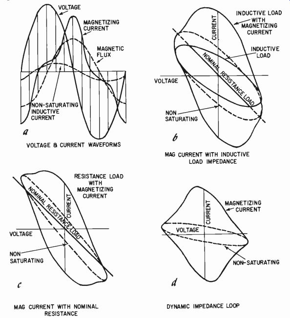
Fig. 427. How saturation current can increase distortion in a practical inductive
load (b), although it may be satisfactory for resistive load (c), or open circuit
(d). Dashed curves indicate effect of a non-saturating transformer for comparison.
When this is combined with the normal resistance load, it may not produce excursion into areas of the transfer characteristic of the amplifier that cause distortion. Similarly, the simple impedance loop for the magnetizing current by itself does not cause excursion into a distortion region. As the amplifier appears to work satisfactorily at the low frequencies where this occurs, it may be concluded that the amplifier will work successfully in this frequency range.
Unfortunately, this omits one very practical possibility--an inductive load combination consisting of the nominal resistance load with an effective series inductance, which is the effective character of all dynamic speakers below their acoustic resonance. This possibility is illustrated in Fig. 427. Note that the combination of inductive load with the magnetizing current produces an excursion which suddenly becomes much more than either the nominal resistance-load arrangement or the magnetizing current loop by itself.
An important thing to check, especially in professional amplifiers, is the stability margin and whether the amplifier behaves satisfactorily on this account at both ends of the frequency response. These require separate consideration due to the different effects they can produce, and because each is essentially independent of the other. For some time it has been thought that square-wave testing is an adequate means of checking transient response. This is not true. It does not even give a guaranteed check of the performance of high-frequency transients.

Fig. 428. Checking waveforms at places other than input and output shows how
square waves can be "faked".
A test consisting of measuring waveforms at points, similar to that shown in Fig. 428, will readily find whether this kind of deviation exists. Notice that the output waveform, like the input, is almost a pure square wave. It comes near enough to a square wave to pass the square wave test, which usually specifies the limits of rise time and deviation (Fig. 429). It is not practical to specify the precise shape of the waveform beyond such limits.

Fig. 429. This illustration shows the quantities of a "square-wave" output
that are usually specified.

Fig. 430. Square-wave testing of an audio amplifier may reveal these waveforms
at various frequencies. The significance of the shapes is indicated in the
illustration.
But to achieve this response some very sharp ringing peaks occur at various other points in this amplifier. This is due to the excessive use of phase compensating capacitors, two of which are shown in this sample circuit, one across the feedback resistor itself and the other across the lower portion of the phase-inverter load (Fig. 428).
If the square wave is keyed, the output waveform will usually show a "rippling" effect. The peaks will bounce in and out of phase until they eventually settle down to the convenient approximation that has been achieved by careful circuit balance. This is no guarantee that the amplifier performs satisfactorily under practical transient conditions.
Square-wave tests have a certain validity, and the significance of several indications is shown in Fig. 430. It is important to check the input waveform with the scope to make sure a square wave is going in. Incidentally, this will also check the ability of the scope to handle a square wave-some do not. Often there is a breakthrough to the horizontal that causes peculiar "jerks" on the wave.
While square waves of appropriate frequency can serve as a quick check of the approximate nature of both magnitude and phase response in the vicinity of low- and high-frequency turnovers, too much trust should not be placed in a good resultant square wave response. It gives absolutely no indication of non linear distortion.
A valid application of the technique is that illustrated in Fig. 429. This is better than a simpler waveform in tracing the round the-loop behavior of a feedback amplifier.

Fig. 431. Input-output comparator response sequence for an amplifier with
the stability margin satisfactorily adjusted. (See also Fig. 403.)
The best approach is to eliminate phase-compensating capacitors, utilizing rolloffs and step circuits in the forward gain characteristic of the amplifier until a satisfactory turnover point at the upper extremity (with feedback applied) produces a 90° phase shift with the attenuation not less than 3 db below the normal 1000-cycle level. This is illustrated by the pattern sequences of Fig. 431. If there is any tendency to peak before the 90° point is reached, or at the 90° point, then the amplifier needs its stability characteristic reworked to eliminate possible high-frequency transient effects.
Performance on low-frequency transients is another question. It has been suggested that tone-burst testing would help. (Fig. 432). This method, using a square-wave-modulated sine wave obtained with the setup of Fig. 433, is useful for finding the things that happen due to changes in performance with the duration of peak signal. It is a dynamic way of finding some of the effects that occur due to supply voltage changes with signal level. It .may also find transient distortion at high frequencies not shown by plain square-waves.
While the former is one form of low-frequency transient, a change in signal level for a duration of several cycles of the lowest component frequency of the signal is also a low-frequency transient. This too may produce one form of distortion that shows up on tone-burst testing.

Fig. 432. Waveform of tone-burst testing signal.
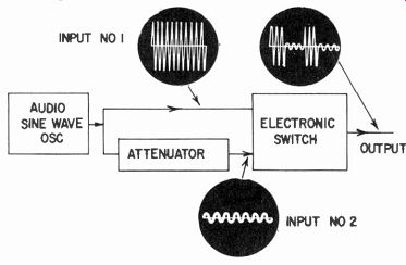
Fig. 433. Basic set-up for generating the tone-burst type of test signal.
Results are assessed, qualitatively or quantitatively, on an oscilloscope.

Fig. 434. Effect of asymmetry of wave form in a non-feedback amplifier; the
low-frequency component introduced is non-oscillatory.
There is another kind of change which does not necessarily involve a change in signal level, although it may sometimes coincide with it. This occurs in program material that has an asymmetrical component to its waveform. Most wind instruments produce such a component. The presence of asymmetry means the acting bias on different stages has to readjust itself after such a change in waveform occurs, from symmetrical to asymmetrical, or back again. (Fig. 434). In old amplifiers (without feedback), this does not cause any particular trouble. It might set off motor-boating, if the amplifier has this kind of instability, but usually it is accompanied by a gradual readjustment of the individual stage biases. This might be reflected in the reading of average plate current in individual tubes, if these were monitored.
[....p116-117]
This means the earlier stages of the amplifier suddenly have to handle many times their normal signal level immediately clipping occurs. For example, a 10% increase in input signal, beyond the clipping point, and assuming 20-db feedback, results in a 100% increase in the signal level handled by the first stage (Fig. 438).
This is a drastic requirement. At the drive stage, for example, there is usually very little margin and this sudden demand for increased handling capacity may exaggerate the clipping which already occurs.
It may also run the amplifier into a sudden overbias condition with the result that, not only clipping occurs, but crossover and other distortions at the same time. It is unnecessary in this guide to go into the possible things that can happen. The important thing is to establish whether an amplifier's performance is satisfactory if a certain permissible overload occurs in the input voltage.
Recommended Reading
1. N. H. Crowhurst, Amplifiers, Norman Price London, 1951.
2. N. H. Crowhurst, Feedback, Norman Price London, 1952.
3. Norman H. Crowhurst, "Frequency Response Audio Amplifiers," Electronic Technician, December, 1956.
4. Mannie Horowitz, "Hum Specification Measurements," Audio, June, 1957.
5. Harold Reed, "More About Hum," Audio, January, 1957.
6. Norman H. Crowhurst, "Why Do Amplifiers Sound Different?" Radio & Television News, March, 1957.
7. Charles P. Boegli, "Transient and Frequency Response in Audio Equipment," Audio Engineering, February, 1954.
8. Norman H. Crowhurst, "A New Approach to Negative Feedback," Audio Engineering, May, 1953.
9. Norman H. Crowhurst, "Unique Relationships," Audio, October, 1955.
10. Norman H. Crowhurst, "Interaction Concept in Feedback Design," Audio, October and November, 1956.
11. Norman H. Crowhurst, "Check List for High-Fidelity Systems," Audiocraft, September, 1957.
12. Norman H. Crowhurst, "Why Feed Back So Far?" RADIO-ELECTRONICS Magazine, September, 1953.
13. Norman H. Crowhurst, "Stabilizing Feedback Amplifiers," RADIO ELECTRONICS Magazine, December, 1956.
14. Norman H. Crowhurst, "Test Equipment For Second-Echelon Ili-Fi Servicing," Electronic Technician, October, 1957. Publishers Ltd., Publishers Ltd., Errors in Hi-Fi