Plotting a Course to the Best Recordings You'll Ever Make: A Guide to the "Geography" of Tape and Recorder Behavior
Cartography by Edward J. Foster (with the B&K Real-Time Analyzer) Baedeker by Robert Long--Robert Long and Edward J. Foster; How-to with graphic aids.
-----------
IF A LITTLE KNOWLEDGE is indeed a dangerous thing, you should use the owner's manual for your tape recorder with the utmost caution. A typical manual will really tell you very little about recording: something about the recorder, perhaps, but very little about tape or, more important, what one manufacturer calls "the symbiosis between recorder and tape." Getting a good recording--a good one--is largely a question of fitting the music (or whatever) into the "space" available in your tape medium. Every recordist knows (or should) that the levels, as shown on the recorder's meters, must not be too high, lest the musical peaks distort, nor too low, lest quiet detail be overwhelmed by inherent noise. But the relationships among overload, sig nal, and noise vary with frequency, as do the recorder's metering characteristics. Without a fairly clear concept of how all these variables re late to each other-the contours of the electro magnetic landscape you're seeking to work with, so to speak-you seldom will get the best possible recording, given the music, the deck, and the tape you're using.
Exploring the Unknown
In order to map the typical landscapes you can en counter, we set up a project unlike any other we've come across before. We chose three tape decks that, although each is an exceptionally fine example of its type, are as different as imagination and available hardware could make them. We also chose tapes that would give us a sampling of divergent types. And we chose three kinds of music: classical orchestra, string quartet, and rock instrumental. Vocal recordings, as such, are not difficult to tape. (Even the acoustic recording medium did a fine job by the human voice.) The instrumental backgrounds, rather than the vocals themselves, are what will pose the problems (if any) for the tape medium; so the instrumental curves shown here can be your guide for vocal recordings as well.
Armed with these variables, we enlisted the participation of that glamour-boy of the equipment testing field, the real-time analyzer. B&K's device divides into frequency bands one-third of an octave wide whatever signal is fed to it and displays (on a screen like that of a TV set) the momentary energy in each of these bands. It can be set to follow each band on an instant-by-instant basis or to hold the highest level in each long enough to read maximum values.
Without such an instrument, some of the information presented here could not have been gathered. We used it extensively as our transit in map ping the contours we will be working with. For one thing, it was invaluable in displaying the maximum instantaneous levels achieved with respect to frequency in the several recordings. The craggy curves thus obtained demonstrate the way in which each musical example makes its demands on the tape medium. The real-time analyzer also made it extremely simple to obtain "response curves" of the tapes' inherent noise. Obviously these data are important in establishing the lower boundary of the working space into which the music must fit.
The upper boundary is a composite, defining maximum useful level as we did in testing cassette tapes a few years ago. [Ed Foster described the test in our March 1973 issue.] The low-frequency portion of the tape overload curve (to at least 1 kHz; the changeover point varies with transport speed, tape, and recorder) represents the recording level at which total harmonic distortion reaches 3%-a commonly accepted "maximum recording level" beyond which distortion tends to rise very rapidly.
But distortion is not the only symptom of tape overload. At higher frequencies a phenomenon known as self-erasure takes over even before distortion becomes excessive. Output from the tape no longer is proportional to input; the tape simply saturates, and adding to the input level actually will reduce the output level through self-erasure.
The upper end of the tape-overload curve there fore represents saturation.
Frequency-response curves should hold little mystery for regular readers. They document the linear-response area of the tape/recorder combi nation and show the degree to which response de parts from the ideal linearity toward the frequency extremes. For test reports on open-reel equipment, response curves are made at -10 VU; for this article we used - 20 VU on all curves (with respect to Ampex zero for the open-reel decks, DIN zero for the cassette deck) to give a better comparative idea of performance between cassettes and open reels. Because of saturation at the high end, response varies with recording level.
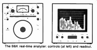
- The B&K real-time analyzer controls (at left) and readout.
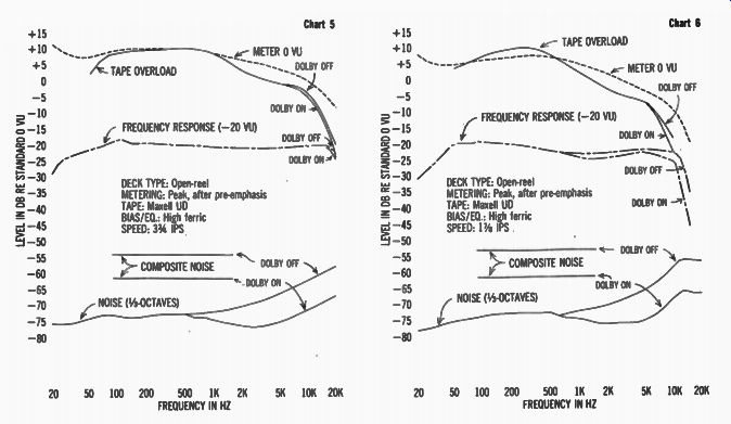
The presentation of both response and overload curves simultaneously shows the relationship between them with unusual clarity. (Note, in particular, the open-reel curves at 1 7/8 ips in Chart 6.) Another variable plotted on our "road maps" is meter action. Three distinct meter types are represented. First there is a true VU (averaging) meter- the type that has been used in professional work for decades. It measures the incoming signal ac cording to a "ballistics" formula that ignores brief peaks (transients), averaging out signal voltages over a long enough time base to allow the recordist's eye to follow the needle's movement.
The second type, represented here on the cassette deck, takes the incoming signal and measures considerably closer to instantaneous values. To prevent excessively fast needle action, the values thus obtained are "held" momentarily by the metering circuit-what is known as a fast-attack, slow-decay characteristic. This usually is called a peak-reading meter--something of a misnomer since it implies the indication of peak voltages, as opposed to rms values for an averaging meter. The difference is strictly one of time: Peak meters will respond to briefer bursts than averaging meters, while they respond identically to steady signals.
The third metering type also is peak-reading, but it measures voltages after the recording pre emphasis is added. The advantage claimed for this system is that it depicts the signals with which the tape actually must cope, rather than the raw in coming signal.
At low levels, you will uncover another boundary of the domain of which you are the master when you operate your recorder: noise. The graphic representation here is a little more complex, and we'll discuss its meaning in a moment.
Our road maps, then, assemble all this information on a single chart for a given combination of recorder, tape, and transport speed, staking out the working limits for that combination. Therefore, not only do the curves show you how the working limits will change when you alter one factor or an other, but by comparing these curves with those for our musical examples you can see just how each type of music must be treated for best possible reproduction.
Obviously we could not include all possible tapes, decks, transport speeds, or musical examples. Those we have used are carefully chosen to typify circumstances commonly experienced by the home recordist; interpolations (and, if necessary, extrapolations) can be made by the reader on the basis of his own equipment and musical tastes.
Before getting into the specifics that our survey yielded, a note is in order about the "composite" indications. In normal musical signals, the tape is not confronted at any given moment with just a single frequency or even a single band of frequencies one-third octave wide. There is a miscellaneous admixture of frequencies, at varying intensities, that assault your recorder's meter and head, and your ear. So any plotting scheme must allow for not only what happens to (and in) individual portions of the spectrum, but how these isolated events will be integrated in the recording and listening processes.
In addition to the third-octave noise curve made with the real-time analyzer, therefore, the recorder graphs show a straight line depicting "composite noise"--a measurement made over the entire spectrum, subjected to what is known as A weighting (which, roughly, corrects these figures for audibility factors so that they generally run about 2 or 3 dB lower than the unweighted type of noise figures shown in our test reports). The composite figures reflect total audible noise-including, to some extent, hum in the electronics of the decks measured. Hum has been excluded from the third-octave curves, which represent tape noise al most exclusively.
The music curves, shown later in the article, likewise have an indication of composite level as well as the frequency breakdown. It is the composite that the meter will read--or the ear will hear--and total dynamic range for any given situation would be measured from the level at which this reading is recorded down to the composite noise measurement.
The whole is, in both music and noise, greater than the sum of the parts. The differences between the curves and the composite values obviously will vary with the spectral distribution of the noise (including the weighting) and with the instrumentation of the loudest musical passages. Music, un like noise, will be totally absent at some frequencies at any given instant, of course.
A Tale of Three Decks
Open Reels, Averaging Meters. We chose the Teac A-7300 to represent this sort of equipment. It is a luxurious unit that in many of its operating features suggests Teac's professional Tascam equipment. It includes three-position switches for adjusting recording equalization and bias, and we made measurements with these switches set at both extremes. (As a matter of fact, we also made measurements at the intermediate settings, but since the differences were minor we chose just three sets that illustrate relatively clear-cut differences.)
---------
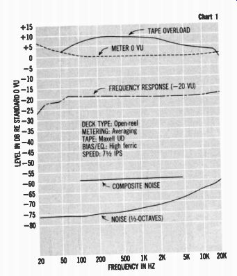
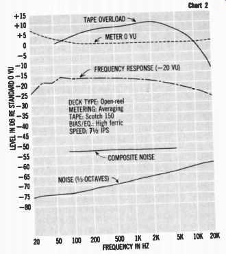
Chart 1 shows the A-7300 used with Maxell UD tape and switched to the "I" (highest) positions for both bias and recording equalization. These positions are specifically adjusted for UD tape, so the response is predictably good. We then chose Scotch 150 tape-which is no longer offered by 3M-as an example of an older tape that, however excellent it may have been in its day, now represents a merely "good" formulation. Chart 2 shows what happened when we measured it with the high bias and equalization settings intended for UD; the results when we used the lowest settings are shown in Chart 3. All of these tests, you'll notice, were made at 7 1/2 ips.
A comparison of the curves made with Scotch 150 tape shows what happens when you use a tape that's a poor match to your recorder. With the higher bias setting the response drops off quite badly as frequency rises; with the lowered bias the response is flattened out somewhat, but even this setting appears to be excessive for this tape. Over load is improved ever so slightly (that is, it is pushed slightly higher at high frequencies) when the bias is lowered, while other properties remain the same. But when you switch to the more "modern" UD tape (with the correct bias and equalization set tings), significant changes occur. The response is flattened to within true high fidelity standards, so that you shouldn't expect to hear any alteration in musical balances. The noise curve, though it reaches exactly the same figure at 20 kHz as those for Scotch 150, is significantly lower elsewhere, while the composite measurement is 5 1/2 dB lower.
In other words, noise will be significantly less audible with UD. But the most interesting result of the tape change is shown in the overload curves. At first glance they may look similar. UD rises almost 10 dB above the 0-VU line; Scotch 150 rises a little higher. If those values alone were the significant ones, it would mean the Scotch could give you a hair more headroom than Maxell and therefore al low you to record at slightly higher levels, partially offsetting its higher noise levels. But notice the frequencies at which maximum headroom occurs. With UD they are squarely in the midrange where, with most music, the greatest signal energy occurs. (To get an idea of what this frequency range sounds like, remember that the A natural to which an orchestra tunes is at or near 440 Hz.) Maximum headroom with 150 is at around 2 kHz- usually a less critical spot in the spectrum. And for close-up percussives like jazz cymbals and for synthesizer music, both of which often contain far more extremely high-frequency energy than you normally would find in conventional pops or classics, the Scotch places severe overload restrictions at the high end, while the Maxell has an overload curve that will take high levels in stride to very high frequencies. These curves show unequivocally the sort of ...
------------
...on the Komische Oper. Even when the Wall went up in 1961, Felsenstein successfully demanded- reportedly from Walter Ulbricht himself-special exemption in order to retain West Berlin residents as employees in any capacity. He shied away from personal publicity, but not long ago he finally capitulated to East German television's long-standing urging to appear on a program during which a studio interviewer and, by telephone, viewers at home threw questions at him. Just as a series of serious illnesses in recent years had made a Felsenstein premiere an even rarer and more eagerly awaited event, his disinclination toward interviews made his television disclosures a rare source of intimate biographical material. "There have been two decisions in my life that I regard as the most important but, in my opinion, not entirely correct," he related. "Originally I studied mechanical engineering at the Institute of Technology in Graz, but only for two semesters. I ran away from there, against the will of my parents, and went into the theater. I enjoyed my dramatic training and became an actor heart and soul-under very bad directors, with the result that I always regarded the director's profession with contempt. I was always glad when during rehearsal the director read the newspaper.
"Then came something unexpected. We were rehearsing Schnitzler's Liebelei, and I had a role I didn't want to give up, but we suddenly had no director and in order to save the play I had to direct it, against my will. How or why I don't know, but it became a success-so great a success that that company unanimously decided that I should re place the same vanished director in staging La Boheme. That was my first opera. I wanted nothing more to do with staging. I was not at all a bad actor, I definitely had a future, but that future got sabotaged by my getting recommended in Basel as a director. Out of a clear sky came a telegram asking me to do a production on trial for the job of chief director there. They engaged me then for both op era and drama. I did not want to become a director. But then I went into all forms of theater-plays, opera, operetta-and I'd like it most of all if I could stage a circus. "There was one more decision that was very, very wrong but unavoidable. With the founding of the Komische Oper, I became director of a theater.
Wherever I had worked before, my productions had made certain demands concerning time, rehearsals, and casting, so that gradually I had to recognize that only having my own house would fulfill my wishes, and so, after three months' reflection, I accepted the invitation .... [It] has brought me a certain success and fulfillment, but I want to emphasize this: I wish I were not the director of a theater. I want simply to create art, not get involved in the thousand other things that keep a theater director busy without pause. If your main profession is the artistic one, it suffers." Felsenstein never had more than twelve operas in the repertory during one season, in contrast with Hamburg and Munich, for instance, which have about sixty. An assistant director took full notes during every performance, and the cast continued rehearsals between performances; as a result, the hundredth presentation of a repertory work often proved fresher and even more vividly alive than opening night. Thanks to generous subsidies, Felsenstein could rehearse a new production, literally, just as long as necessary. He had an elastic rule of thumb that the total amount of rehearsal time should equal the work's performance time multiplied by 300, but he not infrequently exceeded that. Where other houses may allow three weeks, Felsenstein would take months-in the case of his 1974 Carmen production, a total of nine months. Little wonder that a tourist trip he made to the U.S. a few years ago did not lead to any American engagements, although it did eventually add, somewhat atypically. Fiddler on the Roof and I Do! I Do! to the Komische Oper's repertory. Some people have had difficulty resolving the Komische Oper's name with its eclectic repertory.
"The name ... does not refer to opera buff a," Felsenstein explained, "but to Paris' Opera-Comique, an institution founded long ago, in opposition to Paris' Grand Opera, as a house to play not only entirely musical works, but also operatic works involving speech-the original version of Carmen, for example. The name has nothing to do with jolly operas, but with all operas incorporating spoken sections. One has to explain that, otherwise people come expecting something comical and then find, to their astonishment, Otello or Car men." His two principal disciples, Gertz Friedrich in Hamburg and Joachim Herz in Leipzig, have done missionary work in their guest productions in Western Europe and South America for what Felsenstein calls realistisches Musiktheater (realistic musical theater), which means equality of importance between drama and music. And Sarah Cald well of the Boston Opera ranks as the leading exponent of his kind of opera in the U.S. "I believe I coined and propagated the term realistisches Musiktheater," Felsenstein said, "and I have written countless articles and even books about it. ... These principles don't always get fulfilled the way they exist on paper, but in short I should define realistisches Musiktheater as humanly believable and convincing musical stage portrayal. By 'humanly believable' I mean that for the audience a singer must be not audibly and visibly a singer, but rather he must sing because he cannot sufficiently express himself through speech and gesture alone." In Felsenstein's view, a fine voice alone does not ...
--------------
... curves is particularly exact in the critical mid range area from about 200 Hz to beyond 1 kHz, where the energy of musical peaks usually is concentrated. With normal music you can confidently push the peaks right up to the meters' 0-VU indication (but not beyond!): where the music is loaded with highs, it might be better to keep peaks 2 or 3 dB below 0 VU to prevent overload in the region around 5 kHz.
When we switch from 7 1/2 ips to 3 3/4 , several things happen. The increased high-frequency pre emphasis boosts highs going to the meters, causing them to register 0 VU at lower levels for high-frequency signals than they did at 7 1/2. The pre-emphasis also drives the signals farther up against the tape's overload limit (in effect, lowering the over load ceiling with respect to incoming signals at high frequencies), while the reduced tape speed shifts several of the boundaries approximately one octave toward the low-frequency end of the spectrum. The point at which the overload limit starts to drop from its maximum value, and the point at which saturation becomes severe and the overload ceiling begins to drop rapidly, both demonstrate this. And because the saturation curve has been lowered, the point at which response be gins to drop off rapidly has moved from beyond audibility to just below 20 kHz. Similarly, the high-frequency noise curves have shifted a little to the left, hemming in the maximum possible dynamic range from the bottom much as the over load curve does from the top.
While use of the Dolby circuit has little in fluence on any of the curves except that for noise at 7 1/2 ips, at 3 3/4 there is a slight difference in the overload curves as low as 7 kHz (partly because the Dolby circuit compresses highs, moving them upward and closer to overload) and consequently a slight difference in maximum high-frequency response (since overload is beginning to affect response even at -20 VU). All of these properties are much more severe at 1 7/8 ips. And response linearity is more difficult to maintain at this speed, while Dolby action emphasizes the nonlinearities. Because of reduced tape capability at the slower speed and increased demands on the remaining capability (because pre emphasis is higher still), the overload curve is far poorer through the entire top of the frequency range than it was at 3 3/4 ips. The overload curve it self is shown only to 10 kHz, but it re-emerges in the steep drop at the top' end of the response curves.
Noise may appear to improve slightly at the very top of the spectrum, but the flattening of the noise curves above 10 kHz is simply an indication that the combination of magnetic coating, recorded wavelength, and head-gap size is pushed to the limit: At around 12 kHz it exhausts its potential for further useful "work." In terms of pre-Columbian cartography, the frequency has simply sailed off the edge of the world.
• Cassettes, Peak Metering. Cassettes and cassette decks running at 1 7/8 ips will not necessarily give up at the same point as open-reels at that speed.
Head designs differ, for one thing. For another, coatings on cassette tapes bearing the same type designation almost invariably differ-in thickness if nothing else-from their open-reel counterparts.
Sometimes they have little more than the name (and the manufacturer) in common.
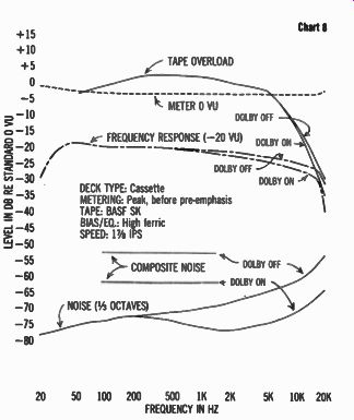
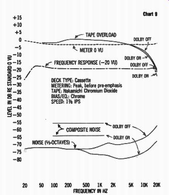
Our choice for a cassette deck, the Nakamichi 1000, demonstrates this, since it is set up for best performance (in the ferric mode) with Maxell UD or Nakamichi EX, which are interchangeable in terms of performance. The 1000 has just the one ferric setting for bias and equalization (the Nakamichi 500 and 550 have an additional, lower bias position for tapes that can profit from it), and we tried it with BASF SK-a modestly priced formulation that has been on the market for some years-as well. And, with bias and equalization switched for chrome, we measured the 1000 with Nakamichi chromium dioxide.
Chart 7 was made with EX. Don't expect any of the results to look like those made on the open-reel decks with UD. The difference is not in the tape so much as in the tape medium, particularly in terms of assumed reference levels and how other behavior patterns relate to them. Whereas traditional open-reel decks allow something like 10 dB of headroom between their 0 VU and the midrange overload point of typical tapes, the DIN 0 VU allows very little: only 2 to 3 dB in this example.
----
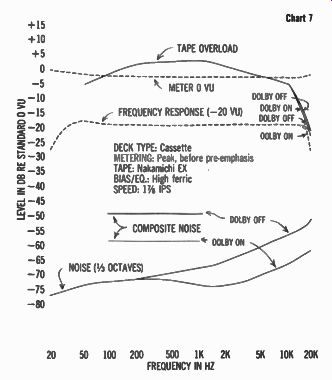
-------- FREQUENCY RESPONSE (-20 VU) DOLBY ON
For that reason cassette deck manufacturers regularly ignore the DIN 0 VU and calibrate their meters somewhat lower to restore at least some of the lost headroom. Nakamichi's 0 VU is 3 dB below DIN 0 VU; hence its metering line lies 3 dB below the zero calibration in our chart. Note that, except in level, it very closely approximates the meter line in the Teac graphs, because both companies (unlike Tandberg) insert the meter ahead of recording pre-emphasis and therefore measure the signal "flat" except for a slight loss in meter-circuit sensitivity at the frequency extremes. But whereas Teac uses averaging meters, Nakamichi's are peak reading. For that reason the 5 dB or so of midband headroom between the meter line and the over load line is ample even though it's only about half that found in the Teac. In other words, an occasional peak of +2 dB or so need not be worried about even though the Nakamichi's meters are reading more nearly instantaneous values. Had Nakamichi used averaging meters, there would be cause for worry about transient spikes, but most cassette decks with averaging meters are adjusted for a still lower 0-VU indication-often 5 or 6 dB below the DIN zero.
This is because the DIN 0-VU reference is much closer to maximum undistorted recorded levels than the standard reference level in open-reel equipment is. Total dynamic range, therefore, is not as great even if the signal-to-noise ratio (measured between the 0-dB line and the composite noise line) is equal. Note that, while the overload line is lower (with respect to 0 dB) than in open reel equipment, it stays relatively high into the up per frequencies, only plummeting beyond 10 kHz.
A carefully chosen match of tape and deck is required if this is to be true in cassette equipment- and if the response curve is to be as flat and as extended as it is in this graph.
Chart 8 shows what happens when, even with an excellent deck, you choose a poorly matched tape. Now the overload line starts to drop rapidly just beyond 5 kHz and the response is anything but flat. If the deck were readjusted to more nearly approximate optimum for SK tape (which some older and less expensive decks already do, of course), the response-particularly that with the Dolby circuit switched on-could be radically improved, and the overload curve should be too.
The SK noise curve already is excellent: about 3 dB better, in the upper frequencies and in the composite measurement, than that for EX. But this virtue is moot without reasonably flat response. And if the deck's bias were lowered to accommodate SK, noise performance should suffer somewhat.
Notice that in Chart 9, made with chrome tape, the noise curves and measurements run about 6 dB better than they do with EX. This does not mean that chrome has inherently lower noise. At extremely low frequencies the noise actually is higher, and at the higher frequencies chrome benefits from its greater playback de-emphasis-
These decks were used for tests:
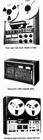
----- Teac open-reel deck, Model A-7300 Nakamichi 1000 cassette
deck Tandberg open-reel deck, Model 9241XD
which pulls down noise along with audio response. That is, the 70-microsecond chrome equalization boosts program highs more in recording and reduces them more in playback.
It can do this because of chrome's higher high frequency overload characteristic. In using the 70 microsecond equalization we trade away part of that high-frequency headroom to buy extra dynamic range. The result of this land-trade deal is an upper limit to our operating area quite similar to that for the ferric EX tape. At 1 kHz, the chrome's overload point is 3 dB below that of EX; elsewhere it is almost as good. Given the Nakamichi's metering characteristics, therefore, you would adjust levels approximately the same way for either tape, though you should be a little more cautious about "recording into the red" with chrome. But even if you set the levels 2 or 3 dB lower for chrome, it still should give you audibly greater dynamic range-that is, quieter tapes for the same listening levels One reason for the excellent noise measurements with the Nakamichi, incidentally, is our test sample's exceptional freedom from hum. This usually occurs at line frequency (60 Hz) or at a harmonic thereof: 120 Hz (the second harmonic) often is the most audible, though its absolute level seldom will be as great as that of the 60-Hz fundamental, and 180 Hz (the third harmonic) some times is present as well. The uncorrected noise spectrum figures on the Teac do show some 120 Hz hum. Those for our sample of the Tandberg prove its 120-Hz hum to be almost completely sup pressed, but there is some 180-Hz hum and a good deal at 60 Hz. Obviously curves that include hum would show differences in this respect from deck to deck-visible differences much greater than those the ear detects from the hum itself. There fore we have included hum in the composite noise figures (on which it has little effect because of the audibility weighting) but not in the frequency curves.
Moving in with Music Now let's examine the demands that actual music makes on our "available recording space." For a symphony-orchestra recording we chose Hoist's The Planets (Leonard Bernstein conducting the New York Philharmonic, Columbia M/MQ 31125). First let's consider the ponderous Jupiter movement, which impresses immediately with its massive scoring. It sounds as though it should be fairly demanding in terms of recorder capability, and it is. Chart A shows that the greatest energy concentration is squarely in that midrange area, around 500 Hz, that we have identified as most critical. But the demands made on the tape medium do not drop off-that is, by 10 dB or more-until we get be low 70 Hz or above 5 kHz. And if we look for the range within which the energy lies at least 15 dB below the 500-Hz maximum, we must go about an octave farther in both directions.
This musical response curve should be fairly typical of late-Romantic, big-orchestra pieces. Re member that the curve represents, simultaneously, the maximum levels in each band. Normally they will be approached during the climaxes, but with out necessarily ever producing exactly the instantaneous energy distribution suggested by the curve. The composite of all frequency bands- what your meters read-measures 3% dB higher at its maximum than any of the frequency bands.
The Uranus movement of The Planets also contains "big" sounds, and it measures quite similarly over most of the range. It does make somewhat greater demands in the range around 8 kHz (which, as the recorder curves show, could be a problem with a poor high-frequency overload characteristic in using one of the older tapes or, in open-reel equipment, a very slow transport speed), but it is the bass that is significantly different. There, an E flat (just below 80 Hz) at the climax actually measures 4i dB higher than the highest level obtained at 500 Hz during the course of the movement. The E flat an octave below (affecting the 40-Hz band) runs almost as high and, be cause of the reduced capabilities one normally can expect of the recording medium at such low frequencies, should be an even greater problem.
The over-all composite level for this movement is only ½ dB higher than that for Jupiter. That is, if you leave your recording level control where it is and record both movements, the meter's maximum swing should be only about 1/2 dB higher when you come to Uranus. But for the extreme demands of Uranus you must avoid over-eagerness in setting that level. The scoring of that movement does put it in the exceptional category-along with, for example, Also sprach Zarathustra, with its large orchestra and organ pedal points.
Much more typical in outline is the Mercury movement, shown in Chart C. On listening to it, you might not think that it would be. The pervading feeling is one of quiet delicacy, with a great deal of high-frequency sparkle. This is deceptive, because the curve shows maximum levels in each band, rather than typical ones. (If it measured typical levels, the curve would be much lower in the midrange and somewhat lower at the high end.) When the climaxes of this movement come, they involve much more conventional scoring than the climaxes of the other two movements. Mercury does not have their roar and crash, produced by al most hyperthyroid activity in the orchestra's brass and percussion sections; it relies more on the basic body of strings and winds. For this reason the frequency distribution of energy in its climax is much more like what one might expect in, say, the symphonies of Mozart and Beethoven. Hence this curve should be a better guide than the other two movements if you are recording classical or high Romantic orchestral works-which, of course, ac count for the majority of the symphonic repertory.
The Mercury curve is quite different-and much easier to record-in comparison with Jupiter and Uranus. Though its maximum point on the frequency curve is only 1/2 dB below that of Jupiter and its over-all composite only 1 dB lower, it makes far less demand at the frequency extremes.
From 5 kHz on up its energy is more than 15 dB lower than the midrange maximum; nothing comes closer than 10 dB of the midrange maximum from 250 Hz down nor within 15 dB of it be low about 60 Hz.
This compares interestingly with the curves in Chart D, for the first and fourth movements of Dvorak's American Quartet, op. 96 (Budapest String Quartet, Columbia M/MQ 32792). Though this disc is cut at a somewhat lower level (the composite measurement for the first movement is 4 dB below that of Mercury, that for the fourth movement 3 dB below it), the curves are virtually identical from 2.5 kHz up. The quartet has a little less energy in the midrange, and of course there is distinctly less energy in the deep bass.
The somewhat lower recording level presumably was chosen for a number of reasons. First, the string quartet has an inherently smaller dynamic range and needn't have its loudest passages pushed as hard against the upper limits of the medium. Second, one tends to listen to a string quartet at lower playback levels; if it were given all the climax power of Ho1st's orchestra, it would sound unnatural. Third, this is a very close-miked recording with a great deal of transient detail in the attacks (the little "noises" that help to characterize the sound of stringed instruments heard from close up), which in energy content resemble the percussives of an orchestra. By backing off somewhat on the level, Columbia may have pre served a little more freshness in these sounds by keeping their transient spikes farther away from overload.
The home recordist would do well to take this example to heart. Where the music recorded doesn't put a premium on maximum recording level you're generally better off if you give up some signal-to-noise ratio in favor of a little more protective headroom. Muddied peaks (from too high a level) may be easier to perceive than added background noise (from one that's too low) under such circumstances.
The curves for Mercury and for the string quartet should be useful for a wide variety of music-including most pops as well as classics-but certainly not for rock. The essential difference is that, whereas conventional music is made with "real" instruments (including the human voice) whose overtone content drops off rapidly beyond the fundamental range of the resonant system by which the tone is produced, rock centers around electronic musical devices that free overtone structure from natural laws. A synthesizer can produce any overtone structure you program it for, and even its fundamentals (the notes actually played on its keyboard) can go far beyond the fundamental range of most acoustic instruments. In addition, there are guitar amplifiers and various electro acoustic devices that can apply the sonic manipulation of the synthesizer to the tones generated by other instruments. The rule is: In rock, expect lots of highs-and lows.
The point is ably made by Chart E, using two of the "Promenade" sections from the Emerson, Lake, & Palmer recording of Pictures at an Exhibition (Cotillion ELP 66666). The first is played on a pipe organ; the second is Greg Lake's arrangement with heavy use of the synthesizer. Same tune, to tally different curves, though the composite is only 2 dB higher for the second "Promenade." The pipe-organ sound is somewhat less demanding at the high end than even the string quartet; at the low end it's more like the symphonic sounds of Jupiter. There is, in fact, not much difference in frequency content at the low end between the two "Promenades"; higher up-and particularly at 10 kHz-they are miles apart.
If you are recording rock, therefore, be cautious.
Not only do you need excellent frequency response if you are to preserve the full impact of the high-level swings into the stratosphere of which the synthesizer and its brethren are uniquely capable, but you must be aware that the flight of these sounds can be grounded by a low overload ceiling even before they reach frequencies where response begins to flag. - Our synthesizer example is by no means extreme (though, as Chart F shows, its peak at 10 kHz is the most extreme of the four sections plotted from Pictures at an Exhibition). Chart F provides curves for two other segments of the Pictures, one of which ("The Great Gates of Kiev") makes heavy demands in the lower midrange and midbass, while the other ("Blues Variation") will pose its problems for the tape medium only in the bass (note the 50-Hz spike) and at the top (near 10 kHz).
----------------
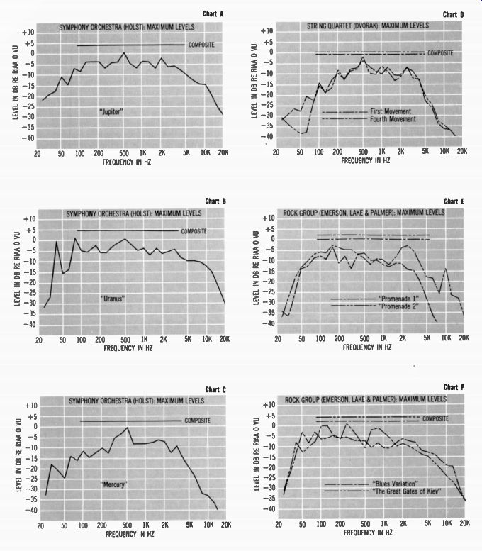
above: Maximum Levels in Our Nine Musical Samples.
Composite musical curves prepared with the B&K analyzer. A, B, and C represent three movements of The Planets by Hoist. Two movements of the Dvorak American Quartet, Op. 96, are shown in D. E and F show sections from Pictures at an Exhibition, rendered by Emerson, Lake, & Palmer.
-------
Plotting a Course
So now we have, on the one hand, our topographical maps of the tape/recorder medium into which we plan to fit our music and, on the other, the lay out of a variety of musical examples. How do you fit them together? We'd suggest you begin with some tracing pa per, or at least some paper thin enough so that you can trace the important curves and then lay one over another. Using this technique, you can derive curves for your recorder and tape, if one of our examples isn't already close to the combination you work with. Actually, most recordists should find that our curves are a reasonably close approximation-close enough for present purposes-and that the nearest match can be used without re drawing. But let's go over the differences that one might find in other conceivable combinations.
In general, most chrome tapes will produce curves almost identical to those shown for the Nakamichi chrome, while most branded ferric tapes (and, if you're interested in really good recordings, you shouldn't be using the cheapies) will resemble either UD (EX in cassettes) or 150 (SK in cassettes that are incorrectly matched to the recorder), or they will fall somewhere in between.
Only the very "hottest" of tapes (like TDK's Audua, BASF LH Super, and Fuji FX) will have the high, arching high-frequency overload characteristic shown for UD and EX. (So will TDK SA, but it is a special case because-though it is a ferric formulation-it should be used much more like chrome.) Most other premium-priced or sub-premium ferric tapes (from companies like Ampex, Memorex, TDK, Capitol, and Columbia) should be expected to have overload curves that don't stay quite as high-at least at high frequencies. The middle-priced and better budget tapes will tend to look more like the 150 /SK curves
The exact curves will vary from these gross generalizations not only with the brand, but with the way your recorder is set up, of course; but these guidelines should give you a rough scale against which you can visualize your available overload curve. And you'll see as we go along that for most music the difference between tapes in this and other respects is not really very great as long as you have a good match between tape and recorder.
It is only in trying to get the very best possible recordings of the more problematic musical exam ples that the differences become really critical.
The tape choice also will affect the noise curves.
As you go down in price, the noise generally will rise much as the headroom lowers. The response will change, too, but here the match between recorder and tape obviously is critical (as Charts 2 and 3 demonstrate). Assuming an excellent match, a little bit (maybe 1 or 2 kHz or response) may be trimmed off the high end of the curve with each downward step in tape price class. And study the influence of Dolby B noise reduction-if you use it-on each of our curves. In boosting high-frequency signals (to keep them above high-frequency noise) the Dolby action will force them closer to overload; where the overload ceiling al ready is low, Dolby action will therefore effectively make it even lower. And it will emphasize any nonlinearity of response above about 500 Hz.
You must remember that we made our measurements with three first-class decks; if yours is not so good, it too will exact a toll in response. In cassette decks, take off about 5 kHz for each halving in price: A $1,000 (three-head) deck may be quite flat out to about 20 kHz, a $500 deck to 15 kHz, a $250 deck to 10 kHz, a $125 cheapie to little better than 5 kHz. The response of cheaper open-reel decks generally won't decline nearly so rapidly with price at 7 1/2 ips, may very roughly approximate the cassette pattern at 3 3/4, and can be truly atrocious at 1 7/8 ips.
Noise, too, will be affected by the quality of the deck in any format. The difference should not be marked until you drop below the moderate price brackets, but in really cheap equipment noise performance can be seriously compromised by electronic noise, hum, and-in battery portables-the use of DC bias.
Again, perhaps you will want to construct a graph representing your own situation, building up your drawing from portions of ours, although it shouldn't be necessary in most cases. In any event a thorough absorption of the principles involved probably will be more helpful in the long run-as a sort of memory bank to which you can make instant reference while you're recording-than the drawings themselves, however accurately they may represent your specifics. But let's see how you might go about adapting our data to an individual, and intentionally oddball, situation.
Let's say you use an open-reel recorder with averaging meters and Dolby processing, plus a run of-the-mill tape roughly comparable to the old Scotch 150, moving at 3 3/4 ips. Not a likely combi nation for a serious recordist, but possible if you have an older recorder (requiring an older tape type), a limited tape budget (requiring the slow transport speed), and an outboard Dolby unit.
Begin with the overload curve. You can trace the midbass portion directly from Chart 3 (the Teac with 150 and reasonably correct bias at 7 1/2 ips) be cause transport speed has little influence on this portion of the curve. But, as you can see in Charts 4 and 5, the overload curve should bend downward somewhat below about 100 Hz when you go from 7 1/2 to 3 3/4. Now before you draw the high portion, study what you would lose in headroom on the Tandberg-without Dolby-when you switch tape speed between these two charts. As previously stated, the whole upper end of the curve shifts to the left by about one octave and bends downward somewhat because of the added pre-emphasis.
Then note the extra bending occasioned by the action of the Dolby circuit. Shift and bend Chart 3's overload curve by approximately the same amounts, and it will be reasonably close to the values you can expect. The metering curve can be copied directly from the Teac, which also uses averaging meters.
The response curve will depend to some extent on the age and condition of your recorder and on the precision with which its bias and equalization settings match the requirements of your tape. This curve won't extend beyond the overload curve you've already drawn in, which will fix the maximum possible upper response limit. For a deck that has a fine separate playback head, the response curve may closely approach this limit; for one that has an inexpensive record/play head, the curve will droop somewhat more rapidly. But if the bias and equalization are closer to perfect than those in the Teac are for 150, the response curve should be flatter at frequencies below the point at which the droop begins. Chances are that, if your taped copies sound slightly dull by comparison with the originals, it is because of a gentle high end rolloff (like that in Chart 3) rather than be cause of the steeper droop at the very top; if your copies sound slightly sibilant, on the other hand, slant your curve upward, instead of downward, above 1 kHz, before beginning that final droop as response approaches overload.
The noise curve would be the most difficult to plot. Again, Chart 3 will give approximate values for your tape at 7 1/2 ips, and the difference between Charts 4 and 5 will show what you lose when you switch to 3 3/4. Actually the difference is very small with the Tandberg/ UD combination. You may experience a greater loss (that is, your noise may be higher), particularly if input-stage noise in your deck is relatively high, since it will be emphasized by the greater high-frequency pre-emphasis at 3 3/4 ips. By following a procedure like that used for overload, you can get the composite noise line and the third-octave noise line-without Dolby. Now draw in the Dolby composite line as far below the non-Dolby line as the distance between the two in Chart 5. And by observing the spacing between the Dolby and non-Dolby lines for third-octave noise in Chart 5, you can likewise sketch in the com parable Dolby curves for your combination.
Whether you feel it necessary to go to these lengths or can confidently use a little eyeball English to make mental correction of curves in the existing graphs, you're now ready to start fitting the music onto the tapes-graphically speaking. In this all-important step, tracing paper is really essential: You must be able to see the tape curves in the background, right through the music curves.
You will find immediately that Charts C and D, which approximate the large majority of musical numbers that you might want to record, fit in very neatly under the overload curves. This is no accident; tape systems have been engineered to accommodate this need. Obviously you don't want any of the craggy "peaks" in the musical contour to press against the limiting ceiling of the overload line, or muddied sound will result. So in these examples it is the energy at around 500 Hz that will determine optimum recording levels.
But how do you set your recording meters so that you will get these levels? That depends on the way your meters work. The B&K real-time analyzer responds to transients much as peak-reading meters do. And in the absence of sharp transients--say, with pipe organ or music for string orchestra--the readings on averaging meters should match data from both averaging meters and the analyzer very closely indeed. It is only when we come to the percussives (or, in speech, "explosive" consonants like T and P) that an averaging meter will conform less closely to actual instantaneous values.
If you have inexpensive averaging meters, you should begin by checking for overshoot. Set your system so that you are feeding a constant signal (interstation noise from FM is a handy source) to your deck and recording it at the meters' 0-VU level. Now switch your SOURCE switch to an unused position (so that you get no input signal) and back again. If when the signal returns the meters go above, say, + 3 VU before settling back to zero, your overshoot is too great for you to get useful meter indication on brief pulses. The reading you see may be too high or too low, depending on the nature of the pulse, and there's no reliable way of judging true values from meter readings.
On a meter with better overshoot damping, pulses of a given level will read lower and lower as they become briefer. With peak-reading meters this generally doesn't happen until the pulse-or the transient, as it's called when it's this brief-is so instantaneous as to defy aural detection of any distortion that it may occasion if it overloads the tape.
Averaging meters will begin to fall off before this extreme brevity is reached, so you must allow some extra headroom wherever the sound is transient-laden. Generally about 6 dB will suffice, but in extreme cases this will not be enough. For example, small bells, when miked close up, produce little midrange energy but a great deal of high-frequency energy in addition to extremely sharp transient spikes. With only average high-frequency overload characteristics in the tape and using averaging meters, you therefore might en counter audible distortion until the recording level is cut back severely; perhaps meter readings could go no higher than -20 VU. But unless you're in the habit of recording ice cream trucks or music boxes you may never encounter anything of this sort. You must, however, listen for transients in whatever you record and be prepared to cut back levels as shown on your averaging meters based on what might be called its percussives quotient.
This would be the equivalent of lowering the music chart with respect to the tape chart. If we take Chart C as representing the music we are recording-say, a string orchestra, which is quite free of loud, sharp percussives-we could place its composite line just below the midrange portion of the overload curve and read, between the meter curve on the tape chart and the composite line on Chart C, the amount of "over-recording" we would need for best possible signal-to-noise. Using Chart 1, you might figure that with transient-free music the loudest passages could read at +9 VU without overloading the tape! And this is true as long as you can be positive that the maximum level you have measured from the music actually is the maximum; let an even higher peak come along, and you're in trouble. So the actual setting of your levels will depend on the exactitude with which you can ascertain maximum levels.
The point is, of course, that we must lower the meter readings to allow for their unresponsiveness to sharp transients-not that we must literally record transient-laden music at a lower level from the tape's point of view with averaging meters.
The ideal recording level is the same no matter what metering system is used; only the meter readings needed to achieve that level will change with the metering system.
And, again, it will depend on what we're calling the percussives quotient, since the machine we're considering has averaging meters. Let's say we decide to keep the levels no higher than +6 VU (which can only be guessed at, of course, because the meters generally won't read much higher than +3 VU) and then we come to a loud pizzicato pas sage that, despite the blurring of the transients (be cause musicians don't play in perfect synchronization), obviously has some peroussive quality.
We may figure that we'd better allow an extra 3 dB for the transients, pulling our maximum allowable meter reading down to about + 3 VU. But then the concertmaster has a pizzicato solo, for which he's provided with a close-up mike and plenty of level boost-putting him on a loudness par with the whole orchestra. The transients now are more sharply defined and, therefore, more meter-defying. Let's allow another 3 dB.
But look at what has happened. We've come right back to the point at which Teac calibrated its meters; we're now reading 0 VU for the loudest passages. This is why standard meters are calibrated this way, in fact-so that there is a midrange headroom of about 10 dB to allow for transients too brief for the meters to read. For progressively sharper transient content, then, you must lower the composite line on the music graph until-for music as percussive as, say, a Dixieland jazz ensemble--it approximately coincides with the meter line.
With peak-reading meters you need make no such allowance. When you place Chart C over Chart 7, you'll find that the former's composite level line can be moved 5 dB above the meter line before the composite line touches the overload line at 500 Hz-the frequency at which maximum music levels occur in this example. Still, a pad of a few dB might be advisable, so you might hold recording levels down to a maximum meter indication of + 2 VU. And when we switch to the more demanding movements of the same composition, as shown in Charts A and B, and set the composite line for each at the same point, we find that the greater high-frequency energy in these movements still doesn't produce crags that come any where near our tape overload line.
Of course the composite lines for the three movements (Charts A through C) of The Planets are not at the same levels. When recording the en tire work, you would set the level for the loudest passage in any movement and leave the recording controls at that setting throughout the piece.
Recording on the Tandberg at 7 1/2 would present no problem in fitting our music into the available recording space on Chart 4. But limits begin to show up when we switch to 3 3 % ips by moving on to Chart 5 and placing that for some "difficult" music-say, Chart A-over it. With the composite line right over the midrange portion of the meter line, we find that the musical energy near 2 kHz comes perilously close to the overload line. But note the shape of the metering curve itself. It is about 3 dB lower at 2 kHz than it is at 500 Hz, meaning that the meters will be about 3 dB more sensitive to that energy peak at 2 kHz and will therefore drive the meter somewhat higher than would be the case had the measurement been made before pre-emphasis.
If we slow the transport speed still further by switching to Chart 6, we find that unless we make allowances for the meters' increased sensitivity at high frequencies we're in real trouble. If we once more place Chart A's composite-level line at about +7 dB on Chart 6, to match the midrange portion of the overload curve, we find that a good deal of the music curve above 1 kHz actually is pushing beyond the overload line into serious distortion.
But the meter curve shows that it will respond with about 5 dB more vigor to energy at 2 kHz than it will at 500 Hz. Since the peak itself is about 3 dB lower than the maximum energy at 500 Hz, a meter that reads 0 VU for the 500-Hz energy might read + 2 VU for the 2-kHz energy. Thus it would force us to lower our levels by about 2 dB (graphically, lowering the composite line from the + 7-dB calibration on Chart 6 to its +5-dB calibration). Lowering the level by another 3 dB for protection (so the composite line falls at + 2 dB on Chart 6) will move our music out of trouble until it approaches 10 kHz where, even if the metering system saves it from overloading once again, the faltering frequency response will probably get it.
Those of you who don't have meters that measure after pre-emphasis-and most people don't- will have to make these corrections for high energy levels at high frequencies yourself. From seeing the corrections automatically introduced by the Tandberg's meters, you should have a good idea what's involved. And remember that, if you have a different open-reel machine with this 1 7 /H ips speed, the performance is likely to be consider ably poorer-no fidelity match even for AM radio, though it may do a fair job with speech or the least demanding of musical signals.
We'll leave it to you to work out what happens when you try to record something even more difficult, like "Promenade 2" from Chart E. As you'll soon discover, it is not recommended at 1 7/8 ips on any open-reel deck. In fact, the more combinations you try and the more you study the details of those combinations-including the ways in which Dolby action alters the potential dynamic range, essentially for the better but not necessarily by the basic 10 dB so often quoted for it--the more clearly you should understand what allowances you can and should make for the music in reading your meters to get the best possible recording with your deck and tape. The object always is to get maximum dynamic range-to "position" the music as high as possible above the noise without forcing it into the overload range of the tape.
As the charts make plain, there is no really simple rule about where the meter should read on a given recorder-no rule of the sort that manufacturers often try to promulgate for their owner's manuals. But still, here's one that may help: When in doubt, use caution. If you're 3 dB below opti mum level settings, it only means that noise will be 3 dB louder with respect to the music than it need be, a barely discernible difference. If you're 3 dB above optimum settings, distortion on the peaks may be several percentage points above what it need be and/or there may be noticeable high-frequency losses. A slightly hissy recording generally is far better than one that sounds mushy, which is just what happens when you overload. But armed with the information in this article, you should be able to steer a course that will help to keep you away from both.
--------
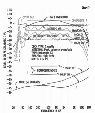
Using the Charts: Trace the music charts and lay them over the tape charts, as explained in the accompanying article. You will find that most music can be recorded on most recorders at levels that drive the meters above 0 vu. You can often dispense with headroom and raise signal levels until they approach tape overload. The colored curves in this illustration represent Uranus from The Planets (Chart B); they are superimposed on the black curves representing the Nakamichi with EX tape (Chart 7).
Since midrange headroom in curve "A" is about 5 1 / 2 dB (the distance from the meter line at -3 dB to overload at about + 2 1 / 2 dB), the recording level might be set so that the loudest passage is 5 1 / 2 dB above the meters' 0-VU indication. The graphic equivalent shows the music's composite line set to coincide with the tape's overload line. This results in an un satisfactory recording with this music because the strong E flats in the bass (40 and 80 Hz) will overload-the peaks pro trude above the overload line.
You might choose to reduce levels on this "difficult" signal until the meters never read above -6 vu. Placing the music's composite line 6 dB below the recorder's meter line (the "B" curves) is the graphic equivalent. But now there is far more room than you really need between the music and tape over load, and the music is down closer to the noise than it need be.
To reduce the audibility of the noise, raise the recording level until the composite line falls on the meter line ("C" curves). The loudest passages now read 0 VU and the music does not impinge on overload; the levels are optimum.
------
(High Fidelity, Feb. 1976)
Also see:
Link | --Link | --Link | --Avid speakers
Classical: Solti's Beethoven symphony package ... Tippett's Child of Our Time ... Marriner's Rossini overtures