3-1. Purpose of Marker Generators
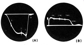
Fig. 3-1. (A) Use of marker pip, to indicate frequencies of important point,
on a tv i-f response curve: a--video i.f., b--sound i.f., c--check point often
specified by manufacturers. (B) Typical tv receiver video-response curve, showing
marker pips every megacycle.
The name "marker generator" is quite descriptive. Marker generators are designed to operate on fixed frequencies, so as to mark these frequencies on a response characteristic. When a response curve of a component or piece of equipment is being swept out by a sweep generator and oscilloscope, the exact limits of the sweep range, or the scale of frequency along the horizontal axis, are not usually known. Even if the approximate limits are known, it is generally difficult and inconvenient to measure off the frequencies of various significant points along the response characteristic. This is particularly true if the frequency change is not linear. An extra signal, which produces a small mark to identify its frequency on the response curve, is of great help in evaluating the curve and making any necessary adjustments.
For example, if a tv receiver is being aligned visually with a sweep generator and oscilloscope, a typical response characteristic may be that shown in Fig. 3-1 (A). Of particular interest in the shape and width of the curve are points a, video i-f frequency; and b, sound i-f frequency.
(The response curve shown is that of the video i-f section of a receiver.) Also important in the observation and adjustment of such a response curve are such points as the peaks, such as mark(d at c, and the minimum point in the "valley" of the curve shown at d.
Figure 3-1 (B) shows a typical response curve for the video-amplifier section of a tv receiver, with a marker at each megacycle. The usefulness of such markers in providing an accurate frequency scale is obvious.
3-2. How a Marker Pip Is Produced
When a steady, unmodulated signal, at a frequency within the pass band of a circuit whose response to be observed, is fed into a tv receiver, this constant-frequency signal will be rectified by the video detector and appear at its output as a d-c voltage. Since direct coupling is frequently used between the video detector and the first video amplifier, the steady r-f signal will merely change the bias on that stage.
Now if a sweep signal for alignment or response observation is applied to the receiver and a response curve traced on an oscilloscope screen, the marker signal will become visible if it is of a frequency within the range through which the sweep generator is sweeping and if it is of the proper relative amplitude.
Let us consider why the sweep signal must be present before the marker is visible. As explained above, a single unmodulated r-f signal, even if within the pass band, becomes merely a steady d-c voltage in the video section, and is not even that after an r-c coupled stage or instrument is passed (such as, for instance, the vertical amplifier of most oscilloscopes). Now suppose the sweep signal is also applied. As the sweep signal passes the frequency of the fixed marker signal, it hetero dynes with it. As the sweep signal frequency approaches that of the marker, the beat signal between them has a relatively high frequency; the beat frequency decreases to zero, and then rises until it disappears again, just as occurs in a radio receiver as we tune through a steady carrier with the beat-frequency oscillator on. However, since the sweep generator signal frequency sweeps rapidly across its range, the heterodyne is produced only momentarily on each sweep and retrace motion. These momentary heterodynes are repeated so rapidly that they blend into one steady indication on the oscilloscope. On an oscilloscope of limited bandwidth, or on a wide-band scope whose response is temporarily reduced by means of a shunt capacitor, an indication of the heterodyne appears for only a few hundred kilocycles on either side of zero beat.
Since this represents only a very narrow spread compared to the entire...
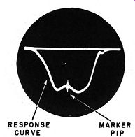
Fig. 3-2. The appearance of a typical marker pip on a response curve.
...response of the circuit, a fairly sharp, well-defined indication appears on the response curve at the frequency of the marker generator.
1. The indication given by a marker on a response curve is called a "pip." The appearance of a pip is shown in Fig. 3-2. The height and broadness of the pip depend upon the amplitude of the marker signal, the response of the oscilloscope, and the relative response of the receiver at the marker frequency. Since the pip is a heterodyne between the marker and sweep signals at the second detector, its size depends upon the amplitudes of both signals in the detector circuit. For example, consider the response curves in the double exposure of Fig. 3-3. When the marker frequency corresponds to a high-response portion of the curve (as at a on the inner curve), not much marker amplitude is required for a substantial indication. However, at the sides and at the edges of the response, as at point b on the outer curve, there is not much receiver response. Therefore, the marker amplitude must be increased to provide indication.
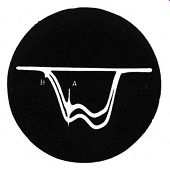
Fig. 3-3. The marker signal must heterodyne with the sweep signal in order
to produce a pip. Where the receiver response is low both signals are weak
at the second detector, thus their beat signal and the pip are weak. That is
why much more marker amplitude is required to produce a pip at b than at a.
[1. Further details about the conditions for producing this indication are given in Section 9. ]
If equipment for sweep analysis is not available, a variable-frequency marker can be used to determine roughly the receiver response. For this it is desirable to have amplitude modulation of the marker carrier. The modulation is turned on, the marker generator is coupled to the receiver, and the resulting audio output from the video section is indicated on an output meter. The frequency of the marker generator is then varied through the response range and the resulting variation of output is noted.
A graph of the output against frequency can be developed by taking readings at regular steps in frequency, as for instance, every tenth or quarter of a megacycle. Of course the input r-f signal must be kept to a low enough level to prevent overloading or age action, or a bias battery added to keep the output-versus-input relation as linear as possible.
3-3. Requirements of a Marker Generator
From the discussion in the previous section, it becomes evident that a good marker generator must have the following qualifications:
1. It must produce a steady unmodulated r-f signal at desirable frequencies in the pass band to be investigated.
2. It must cover the desired frequency range, preferably by continuous variation, or, if crystal controlled, at a sufficient number of frequencies to provide all the information desired.
3. Some method of checking the exact frequency within close limits should be provided, to ensure that the marker indications have proper meaning.
4. The marker frequency should be stable, so that between frequency checks and during tests the frequency will not change to give wrong indications.
5. The amplitude of the marker output voltage should be variable by means of a smooth-variation control and preferably also by a step attenuator.
6. It is desirable in some cases that amplitude modulation by an a-f tone he available, for identification and other purposes.
3-4. Use of A-M Signal Generator for Marker
A study of the requirements listed in the previous section makes it apparent that an ordinary a-m signal generator whose frequency range includes frequencies desired for marking, can be used as a marker generator. The calibrated dial, the output attenuator, and the modulation are all useful for marking purposes as well as in other a-m generator applications. However, the calibration by itself should not be depended upon as final in setting the marker frequencies. Some sort of frequency check should be made to make sure the frequency of each marker 1s correct.
3-5. Marker Generators
Most commercial generators labeled "marker generators" are of the type designed for tv visual response checking. They have variable oscillators which cover the i-f range from 20 to 30 mhz, or from 20 to 50 mhz, and the r-f channel range from 54 to 216 mhz and above. However, a few special laboratory instruments are available for providing markers at various other frequencies.
The controls on marker generators are very similar to those on regular a-m generators, including continuous and step attenuators, modulation on and off switch, frequency range switch, and calibrated dial.
3-6. Calibrators
The requirement that the frequency of the marker be checked and known to be accurate is an important one. For this reason, marker generators are usually accompanied by devices called calibrators. Calibrators are simply crystal oscillators with some additional circuit in which the marker-generator signal can be mixed with the calibrator-oscillator signal or one of its harmonics for comparison. The block diagram of a crystal calibrator is given in Fig. 3-4.
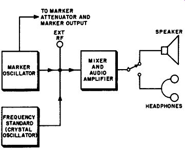
Fig. 3-4. Block diagram expressing the action of a crystal calibrator.
The marker signal beats against harmonics of the crystal-oscillator output. The beat signal is detected by the mixer, amplified, and re produced by speaker or head phones. The marker oscillator is adjusted so that the beat signal is at zero beat. Provision is made on some mode/, for on external marker signal to be checked, at indicated by the terminal "Ext IIF."
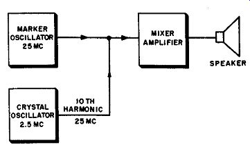
Fig. 3-5. Block diagram giving example of frequency values possible in a
typical case of checking a marker al 25 mhz against the tenth harmonic of a
2.5 mhz crystal oscillator.
The frequency of the crystal oscillator is usually chosen at some even number, such as 100, 250, 500 or 1,000 khz or 2.5, 5, or 10 mhz. Then the harmonics fall at convenient divisions along the calibration scale.
For example, as in Fig. 3-5, the crystal oscillator may be at 2.5 mhz when the marker oscillator is to be checked at 25 mhz. When the marker is tuned close to 25 mhz, its signal will start to beat against the tenth harmonic of the crystal oscillator, which is also at 25 mhz. As additional checks, there will also be another harmonic of the crystal oscillator at 22.5 mhz (ninth harmonic) and another at 27.5 mhz (eleventh harmonic). If the marker frequency dial is even reasonably well calibrated, it can be used to determine quite closely frequencies between two successive 2.5 mhz harmonics, once the harmonic points have been checked. If the calibrated dial readings do not check with the crystal-oscillator harmonics, the difference in each case should be noted, and the readings between harmonics corrected accordingly. Frequently, the marker frequencies to be used fall exactly on a harmonic of the crystal calibrator oscillator.
Then the marker can be set directly on the desired frequency by zero beating it with the crystal-oscillator harmonic, and no reference to dial calibration is necessary, except to make sure that the proper harmonic is being used.
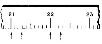
Fig. 3-6. Calibration such as might be used for the tuning dial of a marker
oscillator. This diagram is used in the text to show why two crystal oscillator,
are desirable in making a good check of frequency calibration.
It is desirable to have more than one crystal calibrator frequency, with one frequency much higher than the other. The higher frequency harmonics can be used to place the marker frequency dial fairly close to the proper setting. The lower frequency oscillator harmonics can then be used for the final close check. In fact, usually without the higher frequency check point, it is difficult to identify the proper harmonic.
As a case in point, consider Fig. 3-6. This shows a typical dial calibration, in megacycles, of a marker generator. Suppose a 250-khz oscillator is used to provide calibration check points. Its harmonics will provide signals at each multiple of .25 mhz. However, suppose the dial calibration is in error by the difference between the solid and dotted arrows in the figure. We cannot then tell whether we are beating against the 21.0, the 21.25, o,: the 21.5 mhz harmonic if we have the dial set at the point indicated by the first (left) dotted arrow. But now suppose we have also a crystal oscillator at 1 mhz (1,000 khz). If we switch on this 1 mhz oscillator, and turn off the .25 mhz oscillator, we shall then have check points every megacycle. It is unlikely that the dial calibration in this case is off more than a relatively small part of a megacycle; thus the nearest 1 mhz point can always be identified. Once the 1 mhz point is identified, the 1 mhz oscillator can be shut off and the .25 mhz oscillator turned on. Then starting from the 1 mhz point, we can count .25 mhz points until we come to the one we want. For instance, suppose we want a marker at 21.5 mhz. We turn on the 1-mhz oscillator and turn off the .25 mhz oscillator. We can then identify the 21 mhz point as the nearest harmonic to the 21 mhz dial calibration point. We set the dial to this point, switch back to the 0.25 mhz oscillator, and then tune the generator dial higher until we hear the next harmonic beat, which will be 21.25-mhz; we then continue to tune higher until we beat against the next harmonic, which is the desired 21.5 mhz point.
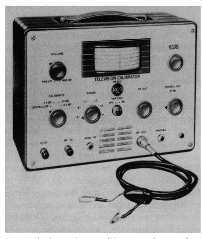
Fig. 3-7. Typical combination marker oscillator and crystal calibrator. Courtesy,
RCA.
A typical marker oscillator and crystal calibrator is illustrated in Fig. 3-7. It covers the i-f range from 19 mhz, and all the vhf tv channels.
The crystal calibrator is completely self-contained, and has .25 mhz, 2.5 mhz, and 4.5 mhz oscillators. A loudspeaker mounted on the front panel reproduces the beat signal between the calibrator harmonics and the marker signal. An external marker or crystal-oscillator signal can be injected into the calibrator through a terminal on the panel; thus other marker signals can also be checked with the same calibrator. There is a suitable attenuator to provide variation of the amplitude of the marker signal.
3-7. Absorption Markers
There is another way to provide marking on a response curve, with out the use of a marker generator. This is known as the absorption method. While the absorption marker is not derived from a generator, its facilities are often provided in a sweep-generator unit.
The principle is simple. A series tuned resonant circuit is connected across the leads from the sweep generator to the receiver. Whenever the sweep-generator frequency sweeps through the marker frequency to which the resonant circuit is tuned, the resonant circuit acts as a very low impedance· and causes a momentary reduction of r-f output until the sweep signal has passed the marker frequency. This produces a noticeable dip in the response curve at the frequency to which the resonant circuit
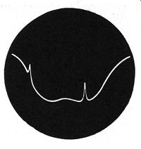
Fig. 3-8. Appearance of absorption marker indications on a response curve.
is tuned. Marker frequencies are adjusted by simply tuning the variable element of the tuned circuit, which is usually equipped with a calibrated dial. The appearance of such absorption markers in a response curve is shown in Fig. 3-8.
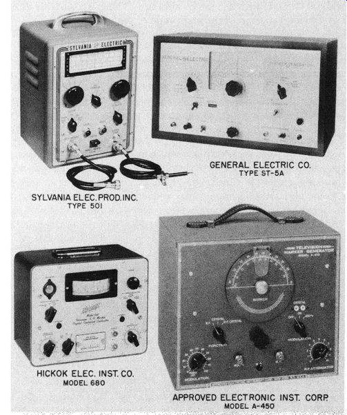
Fig. 3-9. Photograph, of typical, modern marker generator, and calibrators.
Note: The above photo, are reproduced through the courtesy of the manufacturer, indicated.
It is also possible to produce a marker on a response curve by means of a parallel tuned resonant circuit. This circuit is connected in series with the hot lead from the sweep generator to the receiver. Whenever the sweep-generator frequency sweeps through the marker frequency, the parallel-tuned circuit acts as a very high impedance and causes a reduction in r-f output. Under some conditions, a peak rather than a dip may occur at the resonant frequency of the parallel circuit with this hook-up.
This may be due to a sudden reduction in sweep-generator loading at resonance, which causes a pronounced increase in generator output at th marked frequency. In any case, whether a peak or a dip occurs, the indication that should be looked for is a sudden irregularity in the appearance of the response curve at the resonant frequency.