by RICHARD OXLEY
How to use analog techniques and a digital computer to solve second-order differential equations with a few simple algorithms.
By one of those odd coincidences, whilst preparing this article, I came across a war-time bombsight computer in a junk sale. It was, in essence, a mechanical analog computer and must have been extremely difficult to design, manufacture and adjust, particularly as it was mass produced. It served a timely reminder of the traditional difficulty in providing rapid solutions to complex physically related mathematical problems. Consider a mechanical system we all take for granted- the suspension system on cars, consisting of a spring and damper. To describe in detail how this system works under all circumstances is not easy since it requires the solution of a second-order linear differential equation. In terms of automotive engineering, getting the solution wrong can be disastrous because examination of the equation and its solutions reveals that certain combinations of spring and damper characteristics can render the whole system unstable, with potentially lethal results. This is, of course, one of the classic systems studied by generations of engineering students who are taught how to solve the system equation longhand (see example over) but are not expected to do so as a matter of routine, since they are also taught how to simulate the system by means of an analog computer, and thus provide much more useful continuous solutions.
This article describes how small personal computers can be used to solve these ordinary engineering problems. With the correct approach digital simulations of linear systems are relatively easy, with results that can be shown to be mathematically valid on even the humblest of micros.
ANALOG SIMULATION
Most linear differential equations can be simulated by an arrangement of integrators, scalars and summers, and various methods produce the final circuit and correct scaling factors. It must be said however that some of the complexity of the final circuit derived will be due to the sign change introduced by each op-amp and also of course due to the practical limitations of the devices themselves. For instance, the output voltage of an integrator cannot exceed the power supply voltage.
First, let us conveniently assume that the system components are perfect devices. To illustrate this take the equation used in the example, transpose and divide by:
M: _f(t) 121)kKx x M M W
Ignoring scaling factors and sign changes, this results in the analog circuit shown to the right.
The analog simulation of a differential equation leads directly to a very useful and simple method of digital system modeling, since it is possible to write down simple algorithms which model all the components of an analog computer, that is, scaler, summer, integrator, multiplier and even differentiator, although this component rarely needs to be used. Further, just as in the analog computer where components are connected together, algorithms can be connected together to model systems of any complexity.
Before proceeding, it is as well to review how continuous signals as are used in analog systems are represented in digital modeling.
DIGITAL MODELLING OF SIGNALS
Unit steps. In an analog computer, the unit step is simulated by the instantaneous application of a scaled voltage by a switch.
The digital modeling equivalent of this is merely the statement currently being executed in the program:
LET A=X where X is the scaled value.
Continuous signals. The normal interface approach is to use sampling. A sinusoidal signal can be sampled by an a-to-d converter to give a series of numbers in real time for input to a computer at a rate determined by a clock. However, for modeling and simulation purposes, the converter can be replaced by a simple software routine which will produce exactly the same set of numbers, but at a rate determined by the execution speed of the computer. This has no significance, just as the absolute scale of the axes of a graph drawn on paper in no way alters the meaning of the results depicted.
For instance, try the routine:
10 Input "AMPLITUDE": A
20 Input "FREQUENCY": F
30 Input "SAMPLING FREQUENCY": S
40 Q=0
50 X = A*SIN(Q*360*F*S)
60 Q=Q+1
70 PRINT X
80 GOTO 50
This will model a sinewave of frequency F, amplitude A at a regular sampling interval of S by producing an endless stream of numbers to either printer or screen.
DIGITAL MODELLING OF LINEAR COMPONENTS
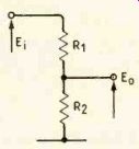
Scaler. A potentiometer divides a signal by a constant which is determined by the position of its wiper on a track, viz:
1Ei
Provided the wiper does not change its position this is the equivalent of division by a constant: Obviously, simple multiplication by the constant shown will produce the desired result:
Y=Xi(R2/jRi + R21).
Y is the instantaneous value of the output signal after being processed by a potential divider with an instantaneous input signal X.
Integrator. The integrating element of an analog computer normally comprises an op-amp with capacitive feedback as shown.
E0 RC JEidt
In practical terms, if a voltage is suddenly applied to the input, the output will change at a linear rate according to the time constant RC and the magnitude of the input voltage.
1Ei EO= R41C Y/s
The digital form of this mechanism is a series of numbers of ascending value separated by a time relationship. The difference in voltage between one sample and the other Is
X = E,*S/ R*C
where S is the sampling interval. To produce a ramp the simple expedient of continuously adding the increment to the previously derived value can be adopted:
X = X + Ei*S/IR*C].
This is known as a recursive function and is the digital equivalent of a linear integrator.
Summer. The other important component used is the op-amp summer. From what has already been given it is pretty obvious that the digital equivalent of that is merely adding two variables, viz:
A=B+C.
Multiplier. Similarly, multiplications of two variables- horrendously difficult in its analog form- is likewise easy:
A = B*C.
Multipliers, incidentally, are used in the solution of non-linear differential equations, often met in systems designed to solve navigation and guidance problems.
===========
CLASSICAL ANALYSIS OF SECOND-ORDER SYSTEM
If a spring is either compressed or extended a distance x by a force:
x« F.'. F=Kx where K is the spring constant (K = Mg/x).
A damper only has an effect when the system moves, in particular the resistive force to movement:
dt«F.'.F=Dx where D is the damping factor.
M T 1-) If a mass is at rest it can only move by an application of a force. That is, the application of a force imparts an acceleration d2x«F
. . F=Mz.
In the case of the spring-mass system, the force producing the acceleration is equal to the sum of the forces acting on the mass. In equilibrium MI=-Kx – Dx +Dx+Kx=O.
When the system is subjected to an applied force, which may be a function of time, Mx + Dx + Kx = f(t).
The classical method for solving practical examples of this mechanical system involves the use of the Laplace operator. Unlike the analog or digital simulator, when differing values for f(t), M, D. and K can be used directly, the two examples given next illustrate how in the classical method different values lead to the use of different mathematical tricks to implement a solution.
----------
EXAMPLE 1
M = 5kg, D = 40N/m/s, K = 80N/m, f(t) = F =
step force of 60N.
MI + Dx + Kx = f(t) 51 + 40x + 80x = 60 ii+8x+16x=12
Applying Laplace:
xs2 + 8xs + 16x = s x(s2 + 8s + 16)= 12 s(s+4)2
To proceed further, the equation should be split into partial fractions such that:
12 _A B C s(s+4)2 s+(s+4)+(s+4)2
.'.12 = A(s +4)2 + BS(s +4) + Cs Put s=0, so A=0.75. Put s=-4, so C=-3.
To find the value of B requires the application of another devious mathematical trick. Equating highest powers: 0 = 0.75 + B, .'. B =-0.75 12 0.75-0.75-3 ..f(t)- 2= + + 2 s s+4 (s+4)
Applying inverse Laplace transforms gives the final general solution:
x(t)=0.75-0.75e-4t-3te-4t
EXAMPLE 2
If the value of D is reduced to five the general solution is radically different. Even the method to find it although basically the same is tediously different.
For the intrepid:
5z + 51( + 80x = 60 z+x+16x=12
By Laplace, xs2 + xs + 16x = 1s and 12 x s(s2+s+16)'
Proceeding by partial fractions:
12-A+ Bs+C 5(52+5+16) 5 s2+s+16 12=0.75(s2+s+ 16)+s(Bs+6). Dating s=0 given A=0.75, while equating coefficients of powers gives B=-0.75, C=-0.75.
x(t)=0'S 5-0.751s2+s+ 161'
The quadratic in the denominator of the second term is factorized by completion of squares:
s+1 x(t)=S 5-0.75((5+0.5)2+1 15.75)-0.75_0.751 s+1 s (s+0.5)2+3.972
The s-term in the numerator of the second term requires some trickery to enable the 'first shift' theory to apply x =0.75_0.75 (s+0.5) 0.5 O S (s+0.52+3.972 (s+0.5)2+3.972)
Applying the inverse transform x(t)=
0.75-0.75(1-e-0 5tcos 3.97t+ 0 5tsin3.97t) 3.97 =0.75[ 1-e-0 5t(cos3.97t+0.126sin 3.97t)].
This result is a damped oscillation with a final settling value of 0.75, shown diagrammatically on page 110. The oscillation has a frequency 3.97/ 2Tr=0.632Hz, a period of 1.58s.
For more about the solution of differential equations using Laplace transforms consult:
Laplace Transforms by K.A. Stroud, Stanley Thornes (Publishers) Ltd.
============
DIGITAL MODEL
Armed with all the algorithms needed to implement a full linear system and returning to the original example, the schematic of an analog computer connected to solve the linear second-order differential equation this time uses the symbols to represent algorithms.
Using the derived algorithms and working from left to right, now write down the program steps required to simulate/model the circuit:
10 X = (F/M)- (D/M*Y)- (K/M*Z) summer 20 Y = (X*S/[R*C]) + Y integrator 30 Z = (Y*S/[R*C]) + Z integrator 40 Print Z
…. where S is sample time, RC is nominal integrator time constant.
It must be remembered that these three equations form a set since they are recursive functions. That is, one equation without the others is meaningless. This is highlighted by the way in which the equations must be incorporated in a program loop. The program incorporating these equations is given in the listing. On a microcomputer it will run until escape is keyed and will output to screen a stream of numbers that represent the action of the real system.
PARALLEL PROGRAMMING
It must be said that the spring/damper used for our example is a very simple second-order system allowing a direct approach to analogs simulation and thence to a digital model. The example solutions show that even with such a simple system obtaining a solution relies on the use of such operator methods as Laplace.
Turning again to the example, it was shown that the displacement of the mass, x, when a step force was applied had the form.
D1 1 x=Rs' (s2+Bs+K)'
The denominator has two parts: 1/s as the Laplace transform of the step function, and 1 s2+Bs+K the Laplace system transfer function or impulse function. Therefore the algorithm previously derived through the direct method forms a digital model of the system transfer function.
When attempting to model complicated systems, the direct approach can become involved. If the system transfer function (or indeed the compound transfer function comprising the system transfer function operated on by the transform of the forcing function) is expanded by partial fractions only three kinds of terms arise, viz: distinct factors, repeated factors and complex conjugate factors, as shown in the panel.
Distinct factor 1 (s+a) 1
Repeated factor (s+a)"
Complex conjugate factor s2+Bs+K
Distinct factor. Remembering that the linear integrator is the equivalent of 1/s, the factor 1/(s+a) results in an exponential rather than a linear output. In fact, it is the equivalent of a simple RC circuit.
Producing such an exponential by algorithms is quite simple since it is a modification of that derived for the linear integrator, viz:
X = X + E,*S/(R*C) linear X = X*(1- IS/(R*C)l) + Ei*S/(R*C) exponential remembering R*C = 1/a.
Repeated factors. The algorithm for the repeated factor is the algorithm for the distinct factor repeated n times, viz
10X = X*(1- S*a) + E,*S*a 20Y = Y*(1- S*a) + X*S*a 30 etc.
where Ei is input stimulus.
Complex conjugate factor. An algorithm that models complex conjugate factors has already been described in the spring/mass example.
Having expanded a complex system equation by means of partial fractions into distinct, repeated and/or complex conjugate factors, a software model would run the algorithms for these in parallel; the full solution would be the simple sum of the algorithms. An example which illustrates this method and models a complex second-order system is given as programming example 2.
DIGITAL FILTERING
I have stuck with the example of the damped spring mass because it leads to a further application of the algorithms that were derived earlier. This system can be considered as a filter. (The suspension system of a car filters out a high proportion of the undulations presented to the wheels by the road surface.) It comes as no surprise then that the analog computer circuit can be used as a general purpose filter which, depending on the particular output connection, acts as a high-pass, low-pass or even bandpass filter.
By outputting either X, Y or Z, a high pass, band-pass or low-pass filter can be modeled whose a.c. characteristics can be predicted. To illustrate this consider the equation for the center frequency of the circuit.
_ 1 Rb,/ 1 fO 27r V R5' V R¡C1R2C2'
If the gain of the two integrators is chosen to be unity:
1/R1C1 = 1/R2C2 = 1 fo becomes 1 R6 R5.
Now this is equivalent to the well-known formula relating to the resonant frequency of the original mechanical system:
fR 2r M
where K is the spring constant, and M is mass.
Comparing diagrams it can be seen that K/M is equivalent to R6/R5, which sets the gain about that particular loop:
This shows incidentally that to speed up or slow down the response of an analog simulation the integrator gain (1/RC) can be changed from unity. For digital modeling the gain of the integrator has less significance and can normally be kept at unity, thus simplifying the algorithms. Conversely, to model such an analog filter to examine its characteristics, then the appropriate time constants for the integrators can be entered into the algorithms directly.
All this provides a useful way of checking the validity of the algorithms. In the original example
F = 60, M = 5, D = 40, K = 80.
fa=2 =0.6366Hz, T=1.57s.
The first programming example shows that these values result in no oscillation because the system is so damped.
However, reducing D to 5 is a different story, and the second trace exhibits damped oscillations with a period of between 1.5 and 1.6s. In fact, the trace exactly models a step function being processed by a low-pass filter with a centre frequency of 0.6366Hz.
This form of recursive digital filter is widely used in the digital implementation of linear control systems. Other forms of digital filter designed to extract continuous signals from random broadband noise can be very complex, relying on statistical techniques.
But for most purposes the recursive digital filter works very well provided that due attention is paid to sampling theory to avoid problems such a aliasing, that is at least two samples per period.
The filtering algorithms can be very useful in some practical applications of micro computers, for instance, control of heating systems by remote sensors. The obvious system to use is shown in the diagram to the right.
Old hands will know that such a system. is liable to all kinds of interference pickup problems from the electricity mains. The sensors will be measuring temperatures that will be varying at a very slow rate but picking up interference at 50Hz and above. Instead of adopting the usual method of hanging big capacitors on everything the problem is avoided by incorporating the above algorithms in the control program to realize a low-pass digital filter.
SOFTWARE OSCILLATION
From the examples given, it will be apparent that under certain circumstances the second-order system as shown will oscillate.
In general, if the damping factor (for the mechanical example) or circuit resistance (for the electrical equivalent) is reduced to zero then the general solution will be a simple sinewave.
Now an algorithm for generating the sine function for input purposes to digital models and filters was given earlier, but of course, it was written in Basic and relies on the host computer containing an algorithm for deter mining the sine of an angle. In some circumstances this facility may not be avail able and so the algorithms derived for the spring-mass (L,C,R) system may be used instead. By choosing appropriate values any frequency may be generated and may, in deed, be faster than the internal routine. The oscillator algorithm then can be used to generate forcing functions for other algorithms which model systems (see second programming example).
This method is very convenient because it is obviously possible by simple software to switch the algorithm on and off at any point in the cycle by loop counting.
Engineers who have struggled with the Heaviside unit step function and the Dirac delta impulse function to show how a complex control system behaves when the input forcing function is an arbitrarily starting sinewave or a pulse will know what an emancipation this is! It is possible also, by resort perhaps to simple arithmetic, to derive algorithms for forcing functions which model other wave forms too--like square waves or sawtooth waves. The output of a bridge rectifier, for example can be modeled by merely ignoring the sign of the sinewave generator algorithm.
In the spring-mass system, if the damping factor B is reduced to zero, the equation becomes 1 sz+K
This is the Laplace transform of 1 sin v K, t.
... where of course, f=1'K/2 pi.
USING THE ALGORITHMS
Care is required when modeling systems to choose a suitable sampling interval. Often surprisingly fast transients are generated by systems, particularly when second or higher order. However, a two low a sampling rate can usually be recognized in the nature of the output from the algorithm since it will show variations in magnitude at the sampling rate. In extreme cases, the output will merely oscillate between rapidly increasing positive and negative values. Trial and error usually determines a suitable value.
However, when the algorithm has been derived from a partial fraction expansion of the system transfer function it may be useful to continue and solve the resultant equation into its cyclic and exponential parts. Since the Laplace transform of the delta Dirac impulse function is 1, the solution gives the impulse response of the system and reveals its frequency components.
It must also be remembered that complex forcing functions will contain frequency components higher than its fundamental.
No matter how slow the system is the output will contain harmonics, admittedly attenuated, of that fundamental. The then becomes a function of the forcing function.
Dick Oxley is a senior systems engineer with British Aerospace Air Weapons Division at Lostock, near Bolton, currently working on infra-red reconnaissance equipment.
EXAMPLE 1: DAMPED SPRUNG MASS
FURTHER READING
Automatic Control Engineering, F.H.Raven, McGraw Hill.
Random Data Analysis and Measurement Procedures, J.S. Bendat &A.G. Personl, Wiley.
Digital Processing of Signals, Gold & Radar, McGraw Hill.
Frequency Analysis, R.B. Randall, Brüel & Kjaer.
Digital Control of Dynamic Systems, G.F. Franklin & J.D. Powerll, Addison-Wesley.
Digital filter design, W.J. Rees, Wireless World Oct. 1976.
Simple digital filters, Palham, Wireless World July 1979.
Analog computing techniques, D.F. Dawe, Wireless World, June/July 1980.
GPIB INTERFACE
T. Segaran's December article on low-cost automated response measurement showed two devices marked 74160 and 74161; these two should be types 75160 and 75161.
EXAMPLE 2: PARALLEL PROGRAMMING
Also see: Within the 68020
==========
(adapted from: Wireless World , Jan. 1987)