By JOULES WATT
Waveform analysis and the Governor of Lower Egypt
“It all started with the French Connection", I said. Once again my discussion group buzzed a little and conjectured about the cryptic beginnings that seemed to grow more and more common in our revisionary topic sessions. By this time I had drawn Fig. 1 on the board. "You might remember that the elementary trigonometric functions have three constants or parameters in their expressions which set the vertical height, the rapidity of oscillation and the position along the axis." Then I asked if Fig. 1 was a sine wave or a cosine wave. The replies varied: some people thought it was a sine wave; others said, "Cosine, because the peak starts nearer the origin." One bright student suggested that, because neither the peak (which would be a plot of cosine) nor the rising zero crossing (which would characterize sine) was at the origin, the plot was neither a sine nor a cosine wave. "On the other hand", he said as an afterthought, "it might be a mixture of both." Later, I appreciated this last suggestion, because it is nearest to our purpose here.
Figure 1 does show a combination of a sine and a cosine wave. If you consider, v=Vsin(wt+4)) (1) t is the independent variable of the function, and v the dependent variable. The V, w and 4) parameters respectively fix the vertical scale, the rapidity with which the graph oscillates as t increases, and whereabouts the sine curve starts relative to the origin.
If the symbols stand for familiar quantities in our subject, we know that v relates to an instantaneous value, usually a voltage. For current, i and I appear in place of the Vs. t indicates time ticking by. V gives the peak value or amplitude and w is the angular frequency, with 4) indicating the phase angle relative to the sine wave origin.
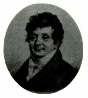
Jean Baptiste Joseph, Baron de Fourier, had a humble start, but gained honors at the military school in Auxerre. Later he joined the staff of the Ecole Normale and then the Polytechnique in Paris.
Fourier went to Egypt with Napoleon, who made him Governor of Lower Egypt after the 1798 Expedition. Returning to France after the withdrawal. he was made Prefect at .Grenoble and then Baron in 1808. He ended up secretary of the Academie des Sciences in 1816 and the following year the Royal Society elected him Fellow.
In 1822, appeared his monumental Theorie Analytique de la Chaleur in which he expounded the theory of trigonometrical series expansion o' periodic functions. He died in 1830.
SINE AND COSINE ARE 'ORTHOGONAL'
You might remember that at about the end of "0" to the start of "A" level maths studies, trig. expansions of compound angles turned up, much to the bane of young students.
Here they are:
sin(A + B) = sinA cosB + cosAsinB
cos(A + B) = cosA cosB + sinAsinB (2)
Use the first relation to expand equation (1),
v = V(sinwtcosd) + coswtsind)). (3)
The sine and cosine of the phase angle 4) must have a right-angled triangle interpretation. This means that from the triangle in Fig. 2 we can write,
v =Visinwt + V2coswt (4)
where V1 and V2 are new amplitudes, both smaller than V, the original. So the single wave in Fig. 1 obviously contains a sine wave and a cosine wave, called its sin and cos components.
Everything about sine compared to cos-sine has a right angle about it--the sides of the triangle from which they arise--the phase angle between them, which is 90° or pi/2 radians--and even the fact that combining them gives the tangent ( = sin4dcos4) which as a trig. function measures how much 'up' for so much 'along'; in other words the slope or gradient).
We are dangerously near j and the work Euler did at this point, a topic we have discussed. In fact, j entering on the scene gives yet another orthogonality relationship.
Orthogonal means 'at right angles to . . . '
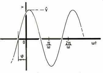
Fig 1. A typical 'sine' wave starting at an arbitrary point, or phase relative
to 0 as shown, has a true sine and cosine component.
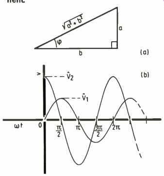
Figure 2. A right angled triangle gives the ordinary definition of the sine
and cosine of an angle we all meet with at school.
Hence,
(b) shows the results of equation (4) and gives us explicitly the sine and cosine components mentioned in the caption to Fig. 1.

FOURIER
Where does the French Connection arise? As you might have guessed, through the work of J. B. Fourier, (see box). Fourier analysis' came into being from his work. In it, he showed not only that the general sinusoidal waveform had a sine and cos component, but all periodic waveforms of any shape also had a whole series of sine and cosine components making them up. Making up a complex waveshape (as certain electronic organ de signs still do) from the basic sin and cos components naturally receives the term Fourier synthesis. Current ways of synthesizing complex waveshapes include using a look-up table in a ROM, repeating the cycle at the fundamental rate you require and using a d-to-a converter. Although this clouds the basic Fourier series components, programming the original table contains the relevant information.
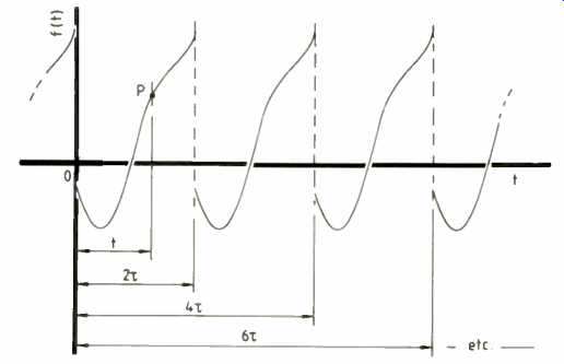
Fig. 3. Any repeating function yields sine and cosine components when Fourier
analyzed.
The period is the shortest interval over which f(t) varies through a complete cycle, shown as 2T here.
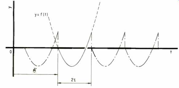
Fig. 4. If you carry out a Fourier analysis on a segment of a non-periodic
function, then the piece is 'reproduced' ad-infinitum. In other words. the
analysis makes the function periodic with the interval of the piece as the
period.
INFINITE SERIES AGAIN
When j was on the agenda', I remember discussing Colin Maclaurin's series, which ‘expanded' a function about the origin, (the point where the independent variable equals zero), so that it could be represented by an infinite series of terms added together.
Perhaps you remember sine and cosine themselves had an infinite series, obtained by that technique. The main difficulty with infinite series methods is that you have to keep an eye on them to see that the series converges to a finite sum.
Fourier used the same method to expand functions, but went further, ending up with an infinite series containing sines and cosines of all harmonic frequencies. Earlier, Daniel Bernoulli had attempted using a similar series in work on how a string vibrates, but was unhappy about the rigor.
Also Leonhard Euler had written a more limited version of such series, but again mistrusted the rigor. Fourier acknowledged Euler's contribution, increased the rigor of the derivations and ended up with integrals, including the ones we still call 'Fourier integrals'. All modern work commemorates his remarkable contributions to mathematical theory under the titles Fourier series and Fourier transform methods.
PERIODIC UPS AND DOWNS
A closer look shows us that such series arise from a special class of functions--the periodic functions. Imagine you are moving along with the independent variable tin the function y = f(t), say, and you look at what y is doing. Your observations might show that y has moved back to, or jumped back to its starting value at some stage in the journey, then went on to repeat the same pattern again.
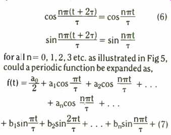
If y keeps doing this, your function is periodic. Sine and cost) typically show periodicity. In fact, they are the archetypes of periodic variations and, as you probably know, the physicists' name for such oscillation is Simple Harmonic Motion. But we term periodic any other function which repeats itself at intervals. From this reasoning, if any arbitrary function f(t) repeats itself every 2T like that shown in Fig. 3 then,
f(t) = f(t + 2T) (5)
The constant 2T is the period.
If any other function, not necessarily periodic, has a piece chopped out of it whose width is 2T, then we can do a Fourier analysis on this segment as if it is repeated indefinitely each way--that is, as if it is periodic, as Fig. 4 shows.
I have made the tacit assumption in talking about oscillations and in using t as a variable, that y is a function of time. But we do not limit Fourier analysis to time variables only: space variables arise in some applications.
Fourier must have asked himself some ting like, "Can any periodic motion, however complicated, be made up the sum of simple motions of the sine and cosine types?" This question asks that, since
. . . which is the usual daunting series expression quoted early in the "Fourier" chapters of textbooks.
Fig. 5. Equations (6) can be hard to visualize. This attempt shows that whatever n is, all the component waves in the cosine and sine harmonic series start at 0. They then go on to repeat the same pattern every 2T.
Of course, as in all these series methods we immediately have to face the awkward question, "What are all those a 0, a1, a2 . . . b1, . . . bn . . . numbers?"
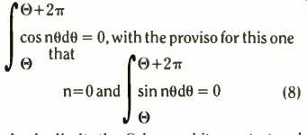
In this instance, as Fourier established, we must use certain integrals to find these coefficients. If you are rusty on evaluating the trigonometrical integrals, a quick glance into a book will remind you that integrating sin and cos over complete periods produces a zero result, because there is as much positive area (above the axis) as negative (below the axis) in the summation,
In the limit, the 0 is an arbitrary start and 2π is the angular period.
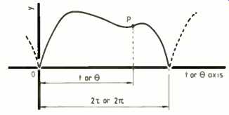
Fig. 6. The fundamental angular periodicity in the trigonometrical functions
amounts to multiples of 2π radians. Generalizing to any interval is useful
and necessary and we do it as shown here.
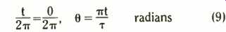
The arguments of the sines and cosines I wrote earlier, for example in equations (7), vary with t. Yet they are angles and I have switched to angles in equations (8). You can see the equivalence of this from t/2 tau being the fraction of the period that 0 to t represents and theta/2π indicating the same fraction of the period, written as an angle. Figure 6 shows that these two fractions describe the same point P and so are equal,
We need one or two more integrals that look even more off-putting but you should find them fairy straightforward when you get down to it
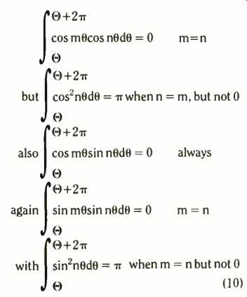
(10)
With these, we can go back and integrate term by term throughout the series, hopefully getting the as as/ and the bs/.
First, simply integrate right through the series with the limits set as before from end to end of the period, Θ to Θ + 2π,
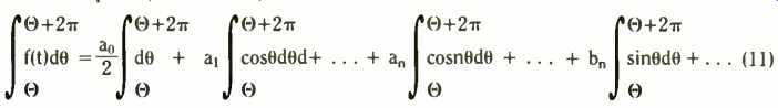
We have assumed f(t) can be integrated. In other words, we do not expect the range of f(t) to go roaring off to infinity, or oscillate infinitely within the domain 2π, so endangering the existence of the integral. Engineering waveform functions certainly do not produce any funny business like that, so we have no worries.
By the first two integrals above, all the cosine and sine integrations on the right vanish away. This leaves only the first term, which is,
(12)
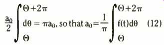
This gives us ao, often called the 'constant' term, or the d.c. term (if the function is an electronic waveform).
We also want the ans and b s, for all the values of n as it steps 1, 2, 3, . . . etc. For the ans, multiply right through the series by cosn_theta and integrate everything again,
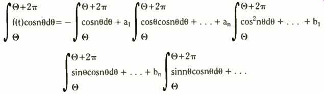
A careful look on the right shows all the integrals equal to zero except the one containing cos^2n_theta, which equals pi.
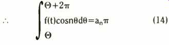
(14)
so we have found the ans.
In the same way, multiplying right through the series with sin n_theta and integrating again, we obtain bn. You will find only the sin2n 0 integration survives to contribute something,
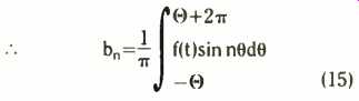
(15)
WE STAY NEAR THE ORIGIN
Most often, instead of the general start, the interval over which the cycle of calculation takes place is 0 to 2π, or to w, so that we take 0 either as 0 or as-w. In other words, we stay around or near to the origin.
We calculated ao separately, but in the cosine part of the series, which gives the ans, ao turns up automatically by putting n = 0 into the integrated result. You might find an occasional problem in doing this--if a denominator went to zero, for example, then the separate calculation for ao would need doing.
What we have assumed is that a periodic function f(t) has a Fourier series. All we can say is if f(t) has a Fourier expansion, then we find the coefficients an and bn as above.
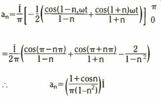
Some of the conditions for the existence of a Fourier series arose from the work of Peter Dirichlet. In a famous theorem he proved, "If a bounded function has at most a finite number of maxima and minima and a finite number of points of discontinuity, without infinite jumps, then the Fourier series of f(t) converges onto f(t) where it is continuous and on to the average of the right and left handed limits of f(t) at each discontinuity." What Dirichlet said means that waves such as those in Fig. 7 have a Fourier series and at each discontinuity the value tends to 1/2(f(t+) + fit-1). Although none of the physically real waveforms with which we have to deal do awkward things, there are relatively simple-looking functions that be have in ways Dirichlet would not have liked, for example,
y = sin 1/t (16)
However small the interval 0 to t, say at the origin, y oscillates infinitely, see Fig. 8, and there is no Fourier series.
R.F.I.
As an example, suppose you had a half-wave rectifier performing in some application.
The radio across the room might produce a buzzing mains hum on the long-wave band every time you had your rectifier system on.
"Ah-ha!, you say, "the jerky diode current turning on and off in the rectification, produces harmonics." This is a typical Fourier situation and we can find the harmonics.
Figure 9 illustrates the usual half-wave rectifier current waveform. Dirichlet would be happy with it; there is only one maximum and one discontinuity (the cusp at the origin) in the domain-pi to pi.
The piecewise function is 0 from-pi to 0 and sin omega t from 0 to pi. Therefore to find the ans, we write
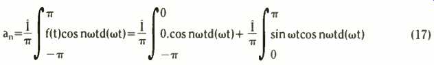
(17)
The first integral on the right contributes nothing, the second gives
(18)
As you can see, we have no result possible for n = 1, and we must do the integral directly.
This shows at = 0. Now let n run. 0, not 1, but 2, 3, 4, 5, and so on, are alright, therefore ao=21/w, al =0, already found, a2--2l/3pi, a3 = 0, a4 =--2l/15pi, as = 0 and so on.
If you go through the calculation for the b s, only one survives and that is b1. All the rest go to 0.
b1 = l/2.
Therefore the final expansion of the half-wave rectifier waveform into its Fourier series is at our disposal,
(19)
The first term is your d.c. component. The second term shows you have a considerable amount of the fundamental a.c. wave pre sent. Then, in the bracket, appear all the harmonics with their amplitudes, that give rise to the radio-frequency interference.
Synthesizing back, term by term, shows how the Fourier components build up the original function. Figure 10 shows that even with only three terms, we get a good approximation to the original half wave, and that not a great deal of energy actually goes into the higher harmonics-which is some relief.
Fig. 7. Dirichelet proved that functions, ever arbitrary and discontinuous
like this one, possess Fourier series. The 'error' in the operation of synthesizing
back by adding a finite number of terms of the series results in oscillations
near the discontinuities. The oscillations persist. which is kr own as the
Gibbs phenomenon (see text). Nevertheless, the synthesized result passes through
the mean points halfway along the discontinuity jumps.
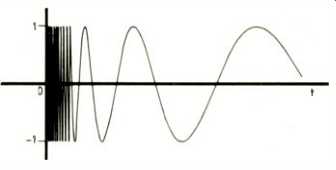
Fig. 8. This function has an infinite number of oscillations in any interval,
however close to the origin. No real physical function behaves like this.
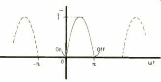
Fig. 9. The typical half sine 'caps' of a rectified a.c. source shown here
illustrate the sharp corners where the diode turns on and off.
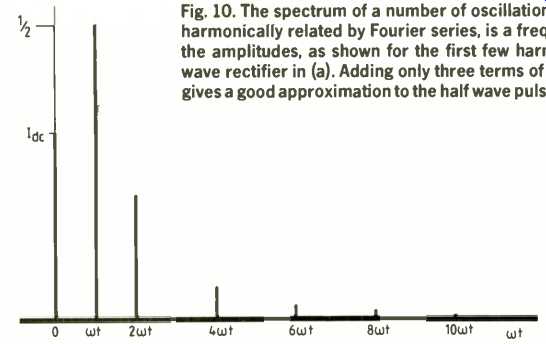
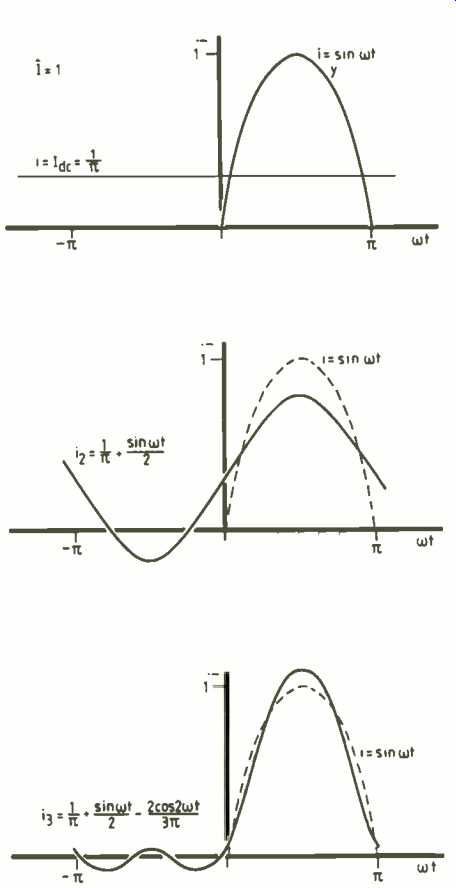
Fig. 10. The spectrum of a number of oscillations, including those harmonically
related by Fourier series, is a frequency axis plot of the amplitudes, as shown
for the first few harmonics of the half wave rectifier in (a). Adding only
three terms of the series already gives a good approximation to the half wave
pulses, as in (b).
THE GIBBS PHENOMENON
On the other hand, the departure from the original waveform is worst near the discontinuities. We see overshooting at these positions. Radio engineers call such transients 'ringing', from their decaying oscillatory nature. Figure 7 shows them. If we take more terms of the Fourier series, the rate of oscillation increases and the amplitude of the overshoot declines somewhat, but even with an infinite number of terms, the over shoot still holds up at some 9% of the jump.
We call this seeming imperfection in the Fourier synthesis of a function, the Gibbs phenomenon. In engineering practice, the energy in the smaller spikes vanishes away and we therefore lose interest in them. But mathematically the stubborn refusal of these spikes to disappear in the limit caused a flurry of interest.
ONLY A START
Of course, I have only scratched the surface of such a large subject. Yet many more detailed textbooks are vague and even mis leading, so that the beginner becomes rapidly confused. However, we have pointed up some of the more intriguing little facts about Fourier, so if you are in the middle of a struggle with learning it all, or about to start, (or even if you are an old hand, but never really got to grips with it!) then go ahead with perhaps a little more confidence.
I will leave you with a little thought. Suppose you had a periodic function like the half-wave rectifier output, but instead of starting the period at -pi through 0 to +π you found the negative start at say, -2π or -3π, but the half sine or whatever still started at 0 and finished at pi? Or further, suppose you saw the half wave at 0 to π, but however far you looked along the axis--both ways--you never found another one. In other words, you only had pulse, at 0 to π.
Would this have a Fourier series? (The first good explanation might enable me to talk the Editor into producing a book token. But you must be just starting as a student--no cheating from Ph.D mathematicians please!)
References
1. Joules Watt, "j" Electronics and Wireless World. September, 1987.
2. J. B. Fourier, Analytical Theory of Heat, English Translation, Freeman. See Sir Harold and Lady Jeffreys, Methods of Mathematical Physics, page 436 for a critical comment on Fourier.
3. G. Stephenson, "Mathematical Methods For Science Students" Chapters 4 and 15. (Longmans).
------------
Also see: Two-dimensional Fourier transforms
==========
(adapted from: Wireless World , Oct. 1987)