By JOULES WATT
Removing DC circuitry and looking at small-signal operation simplifies analysis
My earlier discussion' about parameters turned out to be jumping the gun for a number of readers. If you remember, we considered the generators in the 'black boxes' often used to describe amplifier stages and other blocks in electronic circuits. When knowledgeable, we become complacent about such modeling.
But, in effect, the blandness can be a pitfall. The switch from the real circuit to an equivalent, but different-looking one, which often occurs during discussions about radio and electronics theory, always seems to result in one of those hiccups of understanding, judging from the rather horror-stricken student who said after a lecture, "But the lecturer suddenly short-circuited the supply lines to earth, then drew alternators all over the circuit!" The hardware-schematic to equivalent-circuit jump appears too abstract for most people meeting it for the first time, but seems particularly simple and useful once you know it. This explains the glib way lecturers state it as 'obvious'.
I remember studying "Cathode Ray's" discussion about That Other Valve Equivalent 2, where he introduced the constant-current generator (which turned out to be more suitable for pentodes) in place of the constant-voltage generators that turned up more often in those days. I soon learned that these generators were far from 'constant': they generated the varying signal voltages or currents'.
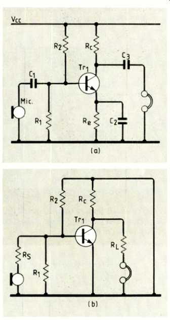
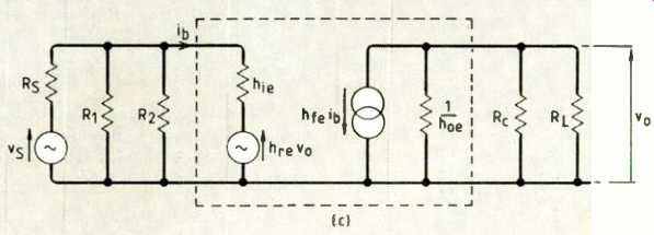
Fig.1. The simple amplifier stage shown at (a), gradually becomes reduced
to the AC small signal equivalent shown in (c), via the step (b) not usually
given in discussions.
MAJOR DIVISION
If you want to analyze or design an amplifier, say, then the overall requirement is either for a simple, single stage or for a multistage system or subsystem. Even in this last case, each stage of the system appears as an entity which you can usually pick out and analyze.
Only in recent times have we found whole subsystems integrated into tiny boxes, in which perhaps the manufacturer has placed a dozen stages working together. This is, of course, the integrated-circuit approach, which enables designers to construct super-systems with many such circuits working together.
Therefore, it would seem that discrete-component designing has decreased and that analyzing the single-stage equivalent circuit might have become obsolete. This is not so in practice, for a couple of reasons:
discretes apparently still get used a great deal; and the integrated devices themselves have an equivalent circuit of the same type as a 'stage' and if you want to know how the inside of the chip works, or even design the stages therein, you still have the full equivalent-circuit approach to cope with. At least some people will need to be experts at such techniques if any more new ICs are ever to come off the production lines.
The trick of the trade is to divide the circuit into two parts and analyze these separately by invoking linearity. Although none of our circuits are linear in their operation, we nevertheless behave as though they were. This enables us to talk about the 'Law of Superposition', which simply means, 'if you work out one solution and then another, the overall result is just the sum of the two'. This means that the two results remain independent and do not interact. In a linear communications system, the two signals pass through independently without cross-modulation, but of course, in a real system, we know that they do.
Mathematically, if the output of a system is, say. V and this is a function of inputs Va and V, and possibly also the temperature T, then,
where v_o is the total change in Vo, va is the increment in Va and so on. We have seen similar expressions before Notice the three terms in this example simply add. They come from straight line segments along the function, or from what amounts to saying the same thing--the linear terms of a Taylor expansion of the function f. Hence the mathematical approximation gives the title to the physical assumption.
From the ability to make this useful simplification, you can assume that the DC bias arrangements which set the operating or Q point and so on, form one 'input' and the AC small signal forms the other. The circuit performance resulting from these can be analyzed entirely separately, then added at the end to get the overall performance--assuming the aforesaid linearity and therefore superposition, applies.
As I already intimated, we knowingly realize that in practice altering the Q point soon alters the AC performance. Also, over driving the circuit with large signals soon results in distortion, cross-modulation, blocking and even shifts in the operating point and bias currents.
Yet this major division of circuits into the DC part and how it operates, together with the AC equivalent with the possibility of its analysis. yields a most fruitful procedure.
AC EQUIVALENT CIRCUIT
As an example, a look at the old, rather obsolescent, single-transistor amplifier stage might revive a few memories. What the books call the 'mid-band' operating region means that the author wants to ignore the reactive effects, with their poles and zeros in the transfer function of the stage. A typical full circuit shown at Fig.1(a), becomes reduced to that in (c).
The way you think through this procedure goes something like this. "Mid-band--let the reactances of the couplers C1 and C3 be zero.
Also let the large capacitor across V to earth in the power supply also offer zero ohms-all the signal frequency". Figure 1(b) results from this thinking, hence the surprise of 'V shorted to earth' when first met.
What you have to see is that with the DC drive removed, the active devices themselves must generate the required power--completely fictitiously of course. With so many equivalents available to simulate this generator action, your skill determines which one to choose in any particular case 3. For good measure, the microphone (in this example) also becomes transformed into an alternator generating the signal v_s.
You might have notice that authors employ the h-parameter set as one of the best descriptors of the small-signal AC performance of the common-emitter stage in Fig. 1. Using these, we finally arrive at the equivalent circuit shown in (c).
Obtaining this equivalent now enables you to take stock. Some books plod on through an analysis of the complete circuit to yield expressions for the voltage gain, the current gain, input resistance, output resistance and perhaps, according to the needs of the moment, one of the various power gains.
Practical engineers note that the resistors at best might be only within ± 5% of their nominal values. The transistor parameters might be even further scattered about the nominal data sheet figures. Further, modern transistors offer very small h. Most often >> R. and R1,. This means the simplification shown in Fig.2 usually gets drawn, ending up with the claim that it will give a working indication.
WHICH GAIN?
I discussed the next problem in an earlier article 3. Whether you want the overall voltage gain, the transconductance gain or any of the others often depends on the transducers used and the duty sought. In this example, we might like to know how many milliamps pass through the head phones for a given sound pressure level at the microphone. The microphone may have its generated e.m.f. versus sound level published in the data sheet. Manufacturers usually note its impedance on the sheet.
We may have an idea of the sound level available from the headphones versus the signal current through them. Therefore the final milliamps out divided by the e.m.f. of the signal source would yield a good performance indicator. This is the transconductance gain,
GT =-iL/v_s
To be strictly accurate, we should call this the 'outer transconductance gain', because you could define an 'inner transconductance gain' iL/vs if you knew vs, which appears across the input terminals instead of the source e.m.f. vs.
BACK OF THE ENVELOPE AGAIN
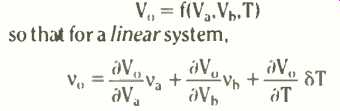
You might be running out of old envelopes if you read these columns, but nevertheless have yet another go on the back of one of them. "as an exercise for the student". Show that the mid-band transconductance gain of the circuit in Fig.1(a), using the simplified equivalent circuit in Fig.2 is,
While deriving this, you should bear in mind the effect of the two current dividers. You will find one of these at the output where current divides between Rc and RL. Only the current through 111, actuates the head phones. The other one occurs where the input signal current divides between RB (which is R1 and R2 in parallel) and h. Only the current through hie operates the transistor. From this discussion you see that we require R_L, << Rc and hie << RB respective ly for maximum gain. If you put these approximations into the equation for GT, you will find it simplifies right down to,
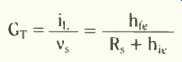
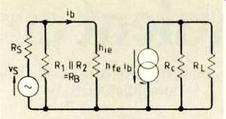
Fig. 2. More often than not, Fig. (c) simplifies even further, by choosing
appropriate approximations which make only a small difference to the final
results.
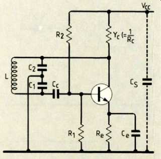
Fig. 3. The well known Colpitts oscillator circuit also can yield its secrets
by means of the equivalent circuit
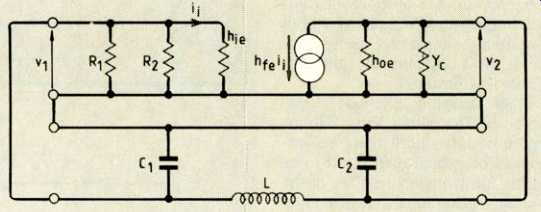
Fig. 4. The first step replaces the transistor with its h-parameter equivalent
as before.
The feedback path via the L-C circuit forms another four terminal network.
TO OSCILLATE OR NOT TO OSCILLATE
How do we know if a certain oscillator circuit will actually start up and continue going? You can go a long way to answer the question by using the same equivalent circuit approach as for the amplifier.
The amplifier operated in the mid-band region for simplicity. A quick think about sine-wave oscillators soon shows that we cannot make the same simplifications in their case, because reactances and resonance are bound to come into the picture as a fundamental part of the frequency-control action. On the other hand, you know just where you want the output frequency to be, so you can make the reactance of the decoupling capacitors zero at that frequency.
In oscillator circuits, there is also a problem with the definition of small signals.
Nearly all of them rely on limitations at the large-signal extremities to keep the amplitude constant. In fact, this causes slight (or perhaps a great deal) of distortion and therefore some harmonic content in the oscillator's output.
We assume at this point in the thinking that the small-signal performance, complete with h-parameters and so forth, will give us information about the start-up condition.
More feedback than this minimum allows the oscillations to grow until the large signal distortion sets in to limit the gain, and therefore prevent further amplitude growth.
Many discussions on oscillators fail to point all this out, so causing more head scratching for students.
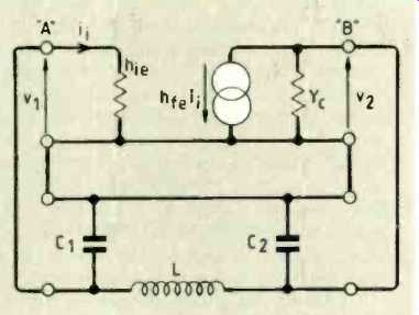
Fig. 5. With the same simplifications as for the amplifier, this is the equivalent
circuit finally analyzed.
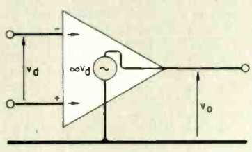
Fig. 6. The op-amp, although a complex integrated circuit, has a very simple
equivalent.
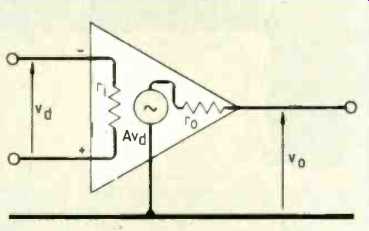
Fig.7. A real op-amp has a slightly more detailed small signal equivalent
(and be cause of internal feedback, this applies to quite large signals also)
which complicates the analysis.
If you look at the oscillator I have chosen in Fig. 3 "Colpitts" should spring to mind, because of the tapped tuning capacitor across L. The AC equivalent circuit immediately gives us Fig. 4 where the transistor has its equivalent h-parameter network and the feedback LC circuit forms another four-terminal network. The networks join up in series at the input and the output of the transistor. A pair of networks in series like this indicates to us that the z-parameters I discussed I turn out to be the most appropriate for the analysis. Like all good rules, such orders should be broken now and then and, in this case, to get round having to convert all the h-parameters to z's, we proceed directly with a nodal analysis instead.
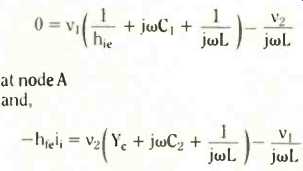
Figure 5 shows a final, simplified, oscillator equivalent circuit assuming that R1 and R2 >> h, and Flo, << Yc. You will notice this is ready for a nodal analysis with v, at node A and v2 at B.
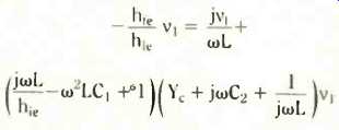
Dare I say it--yet another envelope and you should find the following two equations satisfy Kirchhoff s Current Law at each node,
Now we want to use these to eliminate one of the voltages, say v2, and the current i1.
Current i1 is simple, because i1 = v1/hie. You should discover the final result comes out as
Note that v, cannot be zero all the time, so it can be cancelled right through and you are not dividing by 0. The complex number equation now remaining contains all the information we need for two conditions, as you may remember from "j" 4. These two relationships yield, on the one hand, the frequency of oscillation, and on the other the condition for the circuit to start up and maintain oscillations. You obtain the two expressions by equating the real parts and the imaginary parts of the above equation.
Doing this, you should get for the imaginary parts,
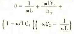
which by dividing through by w (also not equal to 0) tidies up to
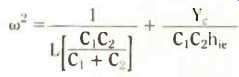
We can write down the final result for the frequency of oscillation by noting that the factor involving C1 and C2 in the first term of the last equation is the effective capacitor, CT, across L in the Colpitts oscillator. Therefore,
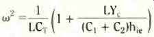
is our grand finale for the frequency of oscillation. We should expect to see the factor outside the bracket, but you might like to have a thought or two about the second term inside the brackets. Obviously (and it is obvious for a change), the frequency of oscillation depends on the transistor parameters (at least on hie) and certainly on the loading of the circuit (Ye). Any resistive output circuit shunts and therefore changes the effective Yc, so altering the frequency.
You should note that this is so even with 'mid-band' non-reactive parameters. When near the high-frequency cut-off of the transistor, where the h-parameters contain imaginary parts and strays contribute, a great increase in reactive terms complicates the issue so much that analytical expressions become virtually unmanageable, although a cad program will enhance the number crunching if you know values of stray capacitances, and so on, to enter.
The final move in this example involves equating the real parts of the above equation. You should obtain
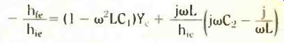
Rearranging a little, you obtain the condition that life must be
Neglect the very small second term in the equation for the frequency we derived above,
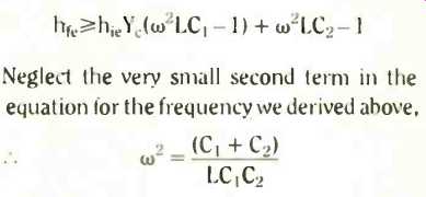
Now you can insert this expression for w2 in the minimum life equation, to end up with a much simplified expression for the maintenance condition,
and we find it gratifying to notice the dimensions all check (pure ratio in this case), so we feel confident of a correct result.
THE SAME WITH ICs
The use of equivalent circuits applies in just the same way to linear integrated circuits such as operational amplifiers, so you can not get away from the idea. The 'first approximation' to an op-amp usually de scribes it as having an infinite input impedance, a zero output impedance and an infinite open-loop gain. We recognize this as the ideal case- never to be obtained in practice, of course, but it gives us a good starting point. The equivalent circuit in Fig. 6 shows how simple it is, and even the humble 741 often becomes elevated to this plane of perfection.
The usual derivation of the closed-loop gains of the inverting and non-inverting amplifier circuits proceed with these simplifying assumptions.
Of course, actual amplifiers depart greatly from these impossible heights. The 741 has a finite input-terminal impedance, a finite output impedance and a large, but certainly not infinite, open-loop gain. It looks like the equivalent circuit in Fig. 7.
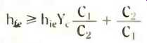
The effect of r, and r with a finite A makes quite a difference to the full analysis, which you might like to try (another envelope...?) For example, consider an inverting amplifier. Figure 8 shows the circuit and the result of working out the voltage gain gives the rather horrific expression,
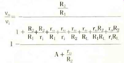
You start off on the journey towards this expression by using Kirchhoff s current law for the summing node (point A on Fig.5) and then do the same thing for the output node (point B). finally eliminating the voltage vt from the two expressions. Tidying up the result gives the above equation.
If r1 -> infinity, ro -> and A -> (what we really mean is if r, >> R1 and R2, and if ro << R1 and R2, together with A 'very large', that is if A> >1 + R2/121) then,

which you may be relieved to see is the ordinary inverting amplifier closed-loop gain relation.
Summing up, we can say equivalent circuits simplify the analysis of stages in amplifiers and oscillators by treating them as linear circuits. By so doing, we can remove the bias or DC circuitry while considering the AC small-signal performance. The operative words are small signal, because the majority of circuits remain linear enough for the approximation only if the signal swings are small.
The discussion I have given only looked at the mid-band region. When you come to consider the full frequency response, things get quite complex (in both senses..., as I hinted in talking about the oscillator. The complex driving point and transfer functions, poles and zeros, bandwidth and stability- all come into the picture, so that the simplifications of the equivalent circuit now become even more appreciated by designers.
Going into all the possibilities, however, is a whole new ball game for another time, as our colleagues across the Atlantic would say.
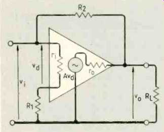
Fig. 8. As noted in Fig.7, the 'less than perfect' op-amp has much more detail
in its analysis, as the result of carrying it out for this circuit shows.
1. Joules Watt, Parameters Electronics and Wireless World. vol.93, No 1612. February 1987.
2. Cathode Ray. That other valve equivalent Wireless World. April 1951.
3. Joules Watt. Voltage or current? Electronics and Wireless World. vol.93. No 1615. May 1987.
4. Joules Watt, j-real thoughts on the imaginary axis. Electronic and Wireless World. vol.93. No 1619. September 1987.
------------
Also see: The maximum power theorem (JOULES WATT)
==========
(adapted from: Wireless World , Dec. 1987)