In this Section, we will study the studio and control facilities for the single channel (monaural) method of broadcasting as practiced by all AM stations and by monaural fm stations. The term "single channel" should not be misinterpreted. This simply means that all microphones and/or tape or disc channels may be mixed as desired, but there is no separation of sound information as to direction of the source.
Transmitter remote control and studio automation facilities are covered in Section 7, although such facilities are just as commonly used for monaural transmission as for stereo or quadraphonic transmission.
6-1. STUDIOS (PRODUCTION)
It must be emphasized here that the majority of broadcast stations today have no concern with production-type studio acoustics, being primarily concerned with disc reproduction and the various tape-system signal sources. However, some stations are heavily scheduled in producing pro grams involving musical pickups, dramatic skits for special events or commercial spots, local panel discussions, etc. These are most often recorded on tape for later use. To provide a useful text, we will cover production facilities and techniques as well as the more common practice of pre-recorded sound sources.
The endeavor to realize high-fidelity transmission of broadcast programs is not new; it has been the goal of at least some engineers since the earliest days of broadcasting. The realization of overall high-fidelity service, however, includes the receiving set in the home, and it has not been until recently that the "average" set in the medium-price market was worthy of the extraordinary efforts of some broadcasters to render high-fidelity service. Conversely, it is apparent that with a good receiver, noticeable differences in fidelity characteristics of different stations within the range of the receiving position now may be noticed by the critical listener.
If the present state of development in broadcast amplifier equipment is taken as the sole criterion, then high-fidelity transmission is truly here.
Frequency response is within 2 dB of the 1000-Hz reference from 30 to 15,000 Hz, and is limited only by wire-line connecting links in AM installations or not at all in fm installations. The noise level at the antenna of the transmitter is at least 60 dB below 100-percent modulation, and the dynamic-range capability is at least 40 dB for AM and 70 dB for fm.
Unfortunately, however, the actual existence of high fidelity depends on many factors other than the of and rf amplifiers associated with the installation. These amplifiers, according to the ideas of some, form the heart of the transmission system insofar as high fidelity is concerned. Actually, they are merely a link in the chain of necessary functions of broadcasting a pro gram and are no more important to fidelity than the other parts of the over all system, as Fig. 6-1 demonstrates.
In order to focus attention on the possible weak links, by eliminating the amplifiers, there remain: program and talent; production technicians responsible for pickup technique; the studio; program producers and announcers; microphones; mixing-room, master-control, and transmitter operators; wire lines; feeder systems and matching units; antennas; and the limitations set by channel bandwidths subject to government regulations. This presents quite a formidable list, and each item is recognizably inferior in performance to the modern amplifier associated with the broadcast installation. To those familiar with broadcasting, however, it may be shown that the weakest links and those which cause most concern at the present time are the studio itself, operating personnel, wire lines, and bandwidth limitations.

Fig. 6-1. Links in the chain involved in putting a program on the air.
The limitations set by wire-line transmission are not serious if considered in relation to the allowable 10-kHz channel of the standard broadcast installation. Formerly, all lines were equalized to 5000 Hz, which is, theoretically, the highest frequency of any effective strength tolerable if adjacent-channel interference is to be prevented. On the other hand, insofar as the relatively small primary coverage area is concerned, the frequency range of modern AM transmitters (12,000 Hz) , when utilized, allows a marked improvement, with class-B and -C service areas suffering from increased cross talk and interference. Although this situation is a deplorable one, it requires little discussion, in that the problem is primarily one under the control of the FCC.
Thus, there remain two factors to be considered, studio design and operating personnel. It is obvious that the broadcaster could possess high-fidelity equipment from microphone to antenna and still not provide high-fidelity service. In the final analysis, the outcome of any program for a given equipment installation depends entirely on the ability of the technical staff responsible for the operating technique. Realizable dynamic range, for instance, which is a highly important factor in high-fidelity transmission, is rarely utilized by station operators. It should be stated, however, that this is not entirely the fault of operators, but is due rather to a combination of factors including an incomplete correlation between the philosophy of dynamic range and compression amplifiers, inadequate visual monitoring indicators for wide dynamic range, and a confusion of ideas existent among personnel as to the amount of dynamic range tolerable in the home receiver for various types of program content. With fm transmission, this problem is even more important. Technical operations are fully explored in Section 11 of this text.
In general, the broadcast studio must meet the following requirements:
1. Freedom from noise, internal or external
2. Freedom from echoes
3. Diffusion of sound, providing a uniform distribution of sound energy throughout the microphone pickup area
4. Freedom from resonance effects
5. Reverberation reduction such that excessive overlapping of successive sound energy of speech articulation or music does not occur
6. Sufficient reverberation such that emphasis of speech and musical overtones is provided to establish a pleasing effect as judged by the listener
In the earliest days of broadcasting, the foremost problems encountered were quite naturally noise and echoes, since studios were simply rectangular rooms with conventional windows and ordinary walls. The first design steps were taken to treat the walls acoustically to prevent echoes and "flutter," and to cover the windows with the same acoustical material. This sufficed for a certain era in broadcasting, provided the operator with control over echoes, and practically isolated the microphone from factory whistles, fire sirens, etc. At that time, this type of studio was entirely adequate to satisfy the fidelity requirements of the program transmission possible with the associated equipment; indeed the electronic amplification of broadcast programs was so much better than the acoustic phonograph that the general public thought of the radio as a realization of true high-fidelity reproduction.
With the advent of the dynamic speaker, microphone improvements, and higher-power and wider-band amplifiers, the scope of fidelity possibilities began to broaden considerably. Signal-to-noise ratio was improved, and higher volumes could be handled in the receiver without distortion, resulting in a greater dynamic-range capability, but at the same time adding to the burden of studio design, since extraneous noises picked up at the studio were now more noticeable in the home receiver. This fact led to the "floating-studio" type of construction.
The following period saw many phenomenal improvements in broadcast equipment in general, such as 100-percent modulation of the transmitter with greatly reduced distortion, improvement in syllabic transmission characteristics, reduction of spurious frequencies and ripple level, greatly reduced noise levels in switching and mixing circuits, and non-microphonic tubes. Yet, strangely enough, studio design remained nearly stagnant over a period of six or seven years, except in isolated cases.
The broadcast engineer found himself faced with many apparent difficulties in rectangular studios. The big factor in a room with parallel walls is the excessive acoustical treatment necessary to overcome the effect of echoes, as mentioned previously. This has resulted, in the past, in extreme high-frequency attenuation and a lack of liveness such that the brilliance of musical programs was completely lacking. The loudness intensity for a given reading on the volume indicator is very low for a studio of this type in comparison with that obtained from a modern studio.
This effect obviously leads into complex operational difficulties, requiring a lower peaking of voice in relation to music to obtain a comparable loudness intensity in the receiver. Furthermore, in this type of studio a number of microphones must be used for a group of performers, since, if a single microphone is employed, a lack of reinforcement of harmonics and overtones of the instruments results in a thin sound lacking in body.
Another difficulty resulting from parallel-wall construction is that the angle of incidence of the wavefronts remains the same no matter how many reflections occur. Due to the acoustical treatment, this reflection (to any great extent) occurs only at the lower frequencies, and the nodes have marked regions of coincident reinforcement, resulting in resonance effects at the lower frequencies; thus conditions that would result in diffuse sound distribution are reduced. It becomes obvious that items 3, 4, and 6, given earlier in the requirements for good acoustics, are lacking in studios of rectangular design. In addition, the high-frequency response so necessary to brilliancy is reduced, effective dynamic range is inadequate, and operational difficulties are numerous. Thus, it is apparent that the studio becomes the weakest link in the high-fidelity chain in the great majority of broad cast installations today. Exceptions, of course, are the main network studios and a few independent stations more production conscious than the main body of independent broadcasters. It is certainly obvious that the large-scale expansion of fm service makes necessary a revolutionary education in studio requirements for the independent station operator, when concerned with local production.
From the foregoing discussion, the difficulties to be overcome may be listed as follows:
1. Lack of sound diffusion
2. Resonance at low frequencies
3. Insufficient reverberation for music
4. High-frequency absorption
5. Critical and multiple microphone placement
6. Operational complexities
The size and dimensions of the studio constitute a certain problem in studio design since an optimum volume per musician in the studio exists.
Reduced to practice, however, this problem becomes one of simply proportioning the studio for a maximum number of musicians expected. This is possible because no difficulty exists in obtaining a good pickup of a small group in a studio designed for a great number of musicians; conversely, because a small room cannot conveniently be "aurally" enlarged, a large band in a small studio presents a difficult problem. Portable hard flats are often used in large studios to enclose a small group of musicians, thus providing the optimum dimensions required for good pickup of a given number of performers.
High-frequency absorption, particularly at frequencies over 5000 Hz, is relatively great. The absorption of sound by air at these frequencies is actually greater than the surface absorption of the studio, even under normal conditions of temperature and relative humidity. It is not possible to con struct a studio having a reverberation time of over 1.2 seconds at 10,000 Hz even with theoretical zero absorptivity of the acoustical treatment. By distributing the reflector surfaces in proximity to the musical instruments, a maximum of diffused, poly-phased high-frequency sound will exist at the microphone without being attenuated injuriously by space behind the instruments. A minimum number of microphones for adequate pickup is necessary under these conditions.
Fig. 6-2 illustrates one method of breaking up parallel surfaces in the pickup area. Both walls and ceilings are interspersed with rounded surfaces to enhance musical sounds without parallel resonance effects. Fig. 6-3 shows Johns-Manville Transite acoustical panels as used in the general-purpose type of studio.

Fig. 6-2. NBC studio A.

Fig. 6-3. Acoustical panels used in a studio.
Fig. 6-4 shows the sound-absorbing characteristics of three materials developed in the acoustical research department of Johns-Manville. By proportioning the amount or adjusting the orientation of these three materials in a studio, the time-frequency curve can be adjusted to any desired contour. This type of studio has the advantage of unlimited pickup area,
but it has the disadvantage of being affected by the size of the studio audience. A great difference in reverberation time exists between a vacant studio and one occupied by a large group of people.

Fig. 6-4. Sound absorbing characteristics of three acoustical materials.
6-2. MATCHING AND BRIDGING PADS AND TECHNIQUES
Due to the complex nature of control and signal routing in typical broadcast systems, fixed attenuation pads are widely used. These devices should be understood before the reader undertakes the study of the main operations center.
The configurations of the two most common types of fixed pads employed in broadcast circuits are shown in Table 6-1. These pads provide constant-impedance loss circuitry generally specified in decibel values of attenuation. The T pad is used where one side of the circuit is grounded or provides a common return. The H pad is used where balanced-to-ground circuitry is involved (the most usual condition).
When the input and output impedances are equal, the series resistors are equal in value. When the input and output impedances differ, the series resistors are of different values on the input and output sides so that the impedance of the pad matches the impedance into which each side works.
This arrangement is termed a taper pad. All pads must be constructed of noninductive elements so that no frequency discrimination occurs.

Table 6-1. Design Data for Fixed Pads
----
For case where Zin = Zout = 600 ohms. For other than 600 ohms (but equal impedances), multiply all resistance values by factor Z,/600 (0.40 for 250 ohms, 0.25 for 150 ohms, 0.083 for 50 ohms.
EIA Resistor Values Nearest to Exact Values
Table 6-1 lists the nearest EIA values of resistors to be used when the input and output impedances are equal to 600 ohms. Note the multiplying factors to be used when the equal impedances are other than 600 ohms.
Observe that the values of the series resistors in the H pad are essentially one-half the values of those in the T pad, since the two sides of the circuit must total the desired amount; R2 is the same in either case.
Due to shunt capacitance effects across large resistance values, it is impractical to obtain attenuation of more than 40 dB in one pad. When greater attenuation is desirable, pads are connected in tandem.

Fig. 6-5. Use of taper pad for feeding 150-ohm line from 600-ohm source.
(A) Notation for T pad. (B) Notation for H pad.
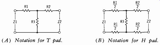
Fig. 6-6. Notation for pads used to match unequal impedances.
Taper Pads
It frequently is necessary to use fixed pads which match unequal impedances. One common example is the isolation pad used to feed the transmitter line (Fig. 6-5 ). Program lines for fm, which are used for wide-band, low-noise service, are often designed to be terminated at both ends in 150 ohms rather than the more common 600-ohm impedance. The pad is used to provide a constant load at all frequencies to the line amplifier, and the repeat coil minimizes induction pickup along the line. The repeat coil is normally operated as a 1:1 transformer, although taps are available for other arrangements. A Faraday screen is used between windings to provide an electrostatic shield which prevents capacitive coupling.
Fig. 6-6A shows the notation used with T pads designed for unequal in put and output impedances. Fig. 6-6B illustrates the H-pad notation. Note that, as before, the series resistance values of the H pad are one-half those of the T pad for a given decibel loss. This notation is different from that used with equal-impedance pads because the series resistors must have different values in the input and output arms due to the requirement of matching unequal impedances.
Step 1: Determine the minimum loss by means of the graph in Fig. 6-7.
This minimum loss is related to the impedance ratio. For example, the impedance ratio of 600/150 is 4/1. The pad must be designed to the nearest decibel loss of an even number (multiple of 2) above this minimum loss value. In the case of a 4/1 ratio, the graph designates approximately 12 dB as the minimum loss. In practice, the design should be for at least a 14-dB loss.
Step 2: To calculate the resistor values, two K factors are required; these may be obtained from Table 6-2. Calculate R1, R2, and R3 as follows:
Ri- (Z1 +Z2)Kl + (Z1- Z2) 2
NOTE: For H pad, divide the result again by 2, per Fig. 6-6B.
R2 _(Z1+Z2)K1-(Z1-Z2) _
NOTE: For H pad, divide the result again by 2, per Fig. 6-6B.
R3 = Z1 + Z2 2K,

Fig. 6-7. Minimum-loss chart.

Table 6-2. Voltage Ratio Values for a Given Loss in Decibels
Take a specific example of a 600/150-ohm pad which should provide a 15-dB loss. From Table 6-2, K1 is 0.697 and K2 is 2.72.
Then:
R1 (600 + 150) (0.697) + (600- 150) 973
_ 486 ohms-
R2 = (600 + 150) (0.697)- (600- 150) _ _ 72 36 ohms 2- 2-
600 + 150 750 R3= 2(2.72)-5.44 =135 ohms
Thus for a T pad (to the nearest EIA values):
R1 = 470 ohms
R2 = 36 ohms
R3 = 130 ohms
For an H pad (to the nearest EIA values) :
R1 = 240 ohms
R2= 18 ohms
R3=130 ohms
NOTE: The R numbers above refer to the configurations of Fig. 6-6.
Bridging Pads
(A) Bridging pad.
Bridging Transformer
Electrostatic Shield (B) Isolation transformer.

Fig. 6-8. Bridging arrangements.
A bridging pad provides a high impedance to the bus to be bridged so that the characteristic impedance is not disturbed, and a matching impedance is seen by the amplifier or unit used. A bridging pad has already been seen in relation to the standard VU meter (Fig. 2-13) .
In practice, a bridging impedance must be at least 10 times the impedance of the circuit to be bridged. This is so that there is no practical attenuation on the bridged circuit itself due to loading. Thus, for a 600-ohm bus, a bridging circuit should present an impedance of at least 6000 ohms to the bus. Consideration must be given to the total number of units or amplifiers likely to be bridged across the circuit, and the bridging impedance of each unit is therefore made as high as possible considering the gain of the amplifier. The gain must be sufficient to make up the bridging loss.
Some amplifiers designed specifically for isolation purposes provide the needed high-impedance input for bridging applications. However, when a standard amplifier input (such as 150 or 600 ohms) must be used, a bridging pad must be inserted between the bus and the amplifier (Fig. 6-8A) .
The shunt resistor (R2) is made equal to the input impedance of the amplifier.
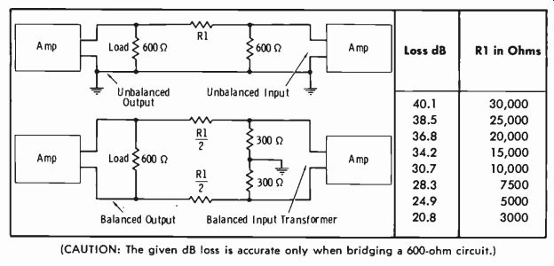
Table 6-3. Value of R1 for Bridging 600-Ohm Circuit
Although the bridging arrangement shown in Fig. 6-8A may be used for either a balanced or unbalanced amplifier, the use of a bridging transformer with an electrostatic shield is preferred for bridging to an unbalanced circuit (Fig. 6-8B) . The loss introduced by such a bridging coil is typically 20 dB.
Table 6-3 shows the two basic types of bridging circuits (unbalanced and balanced), with the values of bridging resistance used for the listed attenuations when the circuit to be bridged is 600 ohms. Bridging resistances down to 3000 ohms have been included. Recall from a previous statement that the minimum bridging resistance should be at least 10 times the impedance of the circuit to be bridged; for 600 ohms, this would be 6000 ohms. The actual loss in the circuit to be bridged may be computed as follows:
Loss in dB = 20 log 2B2B R where,
Br is the bridging input of the pad, R is the impedance of circuit bridged.
Thus for the 3000-ohm bridge mentioned:
dB = 20 log 6000 + 600 6000
= 20 log 1.1
= 0.82 dB, or almost a 1-dB loss in the 600-ohm circuit.
Ideally, the loss in the circuit to be bridged should be under 2 percent.
The problem encountered is not so much the 0.82-dB loss in the bridged circuit, but rather the poor isolation between the 600-ohm circuit and the bridged amplifier. Any form of noise pickup or oscillation that can occur in the input stage of an amplifier would "cross-talk" onto the 600-ohm signal. Also, no more bridging on this line could be accomplished without lowering the total bridging resistance to an excessively low value.
(A) Unbalanced. (B) Balanced.

Fig. 6-9. Combining networks.
Combining Pads
It is frequently necessary to employ branching or combining networks so that more than one feed may be obtained from a single source. For example, a program line might be branched to a monitor line, a test panel, and the program line to the transmitter. Basic arrangements employed for three branches from a single source are illustrated in Fig. 6-9. Build-out resistors (RB) are used to provide isolation between the branch feeds and the source. The value of the build-out resistors is calculated as follows:
RB =N + 1 Z where, RB is the build-out resistor, N is the number of branch output circuits, Z is the circuit impedance.
NOTE: Combining pads are used only between sources of equal impedances.
For a 600-ohm line branching to three circuits of 600 ohms:
RB 600 3 + 1
=0.5 (600)
= 300 ohms
The loss through any two branches is 20 log (N- 1 ) , where N is the total number of circuits. This total includes the source circuit. Thus for the circuits shown in Fig. 6-9:
dB loss = 20 log (4- 1)
=20 log 3
= (20) (0.4771)
=9.54 dB
The loss is the same for either balanced or unbalanced branching pads.
Note, however, that the value of RB is halved for the balanced circuit.
For convenience, Table 6-4 lists the losses for branching pads with one input and up to 10 outputs, when working between impedance values of 600 ohms.
Table 6-4. Loss (dB) for Single-Input, Multiple-Output Pads (Impedance 600/600 Ohms)
6-3. ATTENUATORS (FADERS OR MIXERS)
Variable attenuators serve as faders or mixers in the audio system. They are generally mounted on the operating console. Like the fixed pads de scribed above, the mixer provides a constant input and output impedance, regardless of the amount of attenuation introduced into the path. Two basic physical constructions are used, the rotary type and the vertically-operated type.
The constant input and output impedance of the variable attenuator is achieved by simultaneously increasing the series resistance and decreasing the shunt resistance as the control is turned toward maximum attenuation (and vice-versa for rotation toward minimum attenuation) . This is true for all but the simple ladder-type attenuator, which is described first below.
The ladder type does not provide a complete match at extremes of rotation, and this is its main disadvantage, along with a minimum insertion loss of 6 dB.

Fig. 6-10. Principles of unbalanced ladder attenuator. Rear Cover Removed
Showing Rotary Arm and Contacts of Unbalanced Ladder Attenuator---- Schematic
of Unbalanced Ladder Attenuator
The Unbalanced Ladder
Due to its mechanical simplicity which requires only one row of contacts (Fig. 6-10), the unbalanced ladder attenuator is quite commonly used as a sound mixer. A ladder network is simply a number of cascaded pi resistor sections combined to supply the required terminal impedances and attenuation.
When the ladder-type fader is employed, even though the arm is rotated fully clockwise (minimum attenuation) to the contact at R2, the insertion loss is 6 dB. This minimum insertion loss results from the parallel resistors and the resistor (R4) in the slider-arm circuit. The minimum loss of 6 dB holds true only when the device is operating between like impedances. For example, if the input impedance is 600 ohms and the output impedance is 150 ohms, the resulting impedance ratio of 4 to 1 introduces an additional attenuation of approximately 11 dB (Fig. 6-7) .
Fig. 6-11 illustrates an unbalanced ladder attenuator with a built-in cueing circuit added. As shown, in the extreme attenuation position (maximum counterclockwise) a connection is made to feed the incoming signal to a terminal-board lug for an external cue amplifier. Such attenuators are often provided for turntable and tape inputs to allow proper cue-up of the source, or to fade in the signal at a given cue point without the addition of more switches.

Fig. 6-11. Unbalanced ladder attenuator with cueing position.
The T Attenuator
The bridged T attenuator (Fig. 6-12A) is another unbalanced type of fader popularly used in sound mixers. It requires just two rows of contacts as contrasted to the three rows necessary for the straight T of Fig. 6-12B.
Note that in either case, when the control is turned to the maximum clock wise position (arms on last contact to right) the input is connected directly to the output (with maximum shunt resistance) ; hence, zero insertion loss can be obtained when the device is operated with a 1:1 impedance ratio.
When the straight T attenuator is used, the arm consists of three separate leaves, each of which makes contact with its individual row.
Balanced Attenuators
Fig.. 6-13 presents schematics of the three basic types of balanced attenuators. The balanced ladder (Fig. 6-13A) is simply two unbalanced ladder networks inserted in the two sides of the line and coupled together on a common shaft. Like the unbalanced ladder, this attenuator has a minimum insertion loss of 6 dB.

Fig. 6-12. Types of T attenuators. (A) Bridged T. (B) Straight T.
The bridged H attenuator (Fig. 6-13B) is simply two bridged T net works mounted on a common shaft. Each section requires two rows of contacts; hence two units are mounted in tandem and operated by the common shaft. The front and rear units are securely fastened together within a totally enclosed dust cover. By depressing release springs located on the sides, the rear section can be removed to expose the contacts of both sections for cleaning.
The balanced H attenuator (Fig. 6-13C) consists of two straight T units mounted in tandem. Three variable resistors are used to form the T net work in each section, and the sections are connected to form a balanced H.
Each section requires three rows of contacts.
The bridged H and balanced H attenuators provide zero insertion loss when operated with a 1:1 impedance ratio, just as is true for the unbalanced T attenuators.
Low-Level Mixer Circuits
Low-level mixing is often employed in the simpler control consoles (six channels or fewer) such as those sometimes used in remote locations or as subassemblies in larger installations. For six-channel mixers, the T-type attenuator is normally used to avoid the extra 6-dB minimum insertion loss of the simpler ladder type. Four-channel mixers often employ the ladder type for channel mixers and a T type for the master level control (when used).
Low-level mixing simply means the input signals pass through the mixing network prior to amplification. Fig. 6-14 shows the basic principles of low-level mixing circuits. This example is an unbalanced parallel type of mixer with a 1:1 impedance ratio. Most larger control consoles employ high-level mixing, which means an individual attenuator is used between amplifiers for each channel.
As given in Fig. 6-14, the minimum loss for this type of mixing circuit is 20 log N, where N is the number of channels. If the ladder-type mixer is used, the insertion loss of 6 dB must be added to this computation. The data of Fig. 6-14 are for a 1:1 impedance ratio such as 600:600, 150:150, etc.
The value of the build-out resistor (R) is dependent on both the source impedance (which in this case is also the output impedance) and the number of channels employed. The table of values of R in Fig. 6-14 is a "quick computation" list for reference.
Variable attenuators are purchased from a manufacturer, but the user must know how to combine these networks when building his own gear, such as portable sound mixers or an auxiliary mixing panel. The data of Fig. 6-14 (for 1:1 impedance ratio) and Fig. 6-15 ( for taper attenuators between unlike impedances) are required for this purpose.
The diagram in Table 6-5 gives the basic design parameters for allowable mixer loss to a given amplifier or preamplifier. For convenience in application, Table 6-5 lists the actual mixer loss for the number of channels indicated in the left column.
An impedance-matching transformer sometimes is used in the position of the master gain control of Figs. 6-14 and 6-15 to feed a following amplifier. The master gain control then follows this amplifier to feed the program line amplifier.


Fig. 6-13. Balanced attenuators. (A) Balanced ladder. (B) Bridged H. (C)
Balanced H.
A side view of a typical vertical-type attenuator is shown in the drawing of Fig. 6-16. Sometimes the in-out and common terminals are brought to a receptacle to allow plug-in of units.
6-4. EQUALIZERS
Equalization as applied to tape recording and playback has already been discussed. Based on the same principle are equalizer networks for long lines ( studio to transmitter, network distribution, remote installations, etc.) and special equalizers used in production-type equipment for special effects, frequency emphasis or de-emphasis for echo use, etc.

Fig. 6-14. Low-level mixing circuit, 1:1 impedance ratio.

Table 6-5. Mixer Loss

Fig. 6-15. Low-level mixing circuit, unequal impedances.

Fig. 6-16. Side view of typical vertical attenuator.
Line Equalizers
Telephone lines used for the distribution of broadcast signals have a gradual rolloff off high-frequency response due to series inductance and shunt capacitance. Equalizers are installed by the telephone company at the receiving end of the line or cable, such as at the transmitter for studio-to- transmitter paths, or incoming network or remote lines at the studio. It is also desirable to have an adjustable line equalizer at the studio for use on remote pickups for which the lowest-priced line service may be requested for a "one-time" pickup ( which means the line is not equalized by the telephone company) .
Although most commercial line equalizers contain multiple sections for critical equalization, Fig. 6-17 illustrates the principle of operation. The LC network is normally made to resonate at a frequency slightly above the highest frequency of concern, such as 8 kHz for an AM line or 15 kHz for an fm line. In noncritical remote pickups where only voice signals are involved, this frequency can be made about 5 kHz. The value of adjustable resistance R depends on the length of the line. The longer the line, the more equalization is required; thus a longer line needs less resistance than a shorter line. This is to emphasize that the variable resistance determines the magnitude of equalization; if R is made a short circuit, the maximum equalization is in effect. As the frequency is increased, the impedance of the shunt circuit increases; hence the response on the line is increased.
Line Equalizer
Line Input C L- Input to From- Terminal Repeat Coil Gear

Fig. 6-17. Simplified representation of line equalizer.
Conversely, as the frequency is decreased, less effective impedance is presented by the shunt circuit, and lower frequencies are attenuated. The circuit is so designed that a "shelf" is provided such that equalization starts at the frequency where rolloff starts on the particular line involved. The average value of the "shelf" is around 1000 Hz.
The best way to visualize a line equalizer is to consider it as an attenuator at lower frequencies in the passband, with characteristics such that the response across the entire passband is flat. This explains the inevitable insertion loss of the equalizer, which then obviously depends on length of line, wire size, and frequency band to be equalized. The average value of this insertion loss in practice lies between 30 and 40 dB. A booster or line amplifier with a resistive input terminating network to load the equalizer is required to compensate for this loss.
Fig. 6-18. Typical control module for individual channel. Equalization Controls Mic or Line Selector Attenuator Switch Vertical-Type Level Control
Production Equalizers
Professional recording, production-type broadcasting, and sound-reinforcement systems incorporate many types of special equalizers. Fig. 6-18 illustrates a typical control-panel module for an individual channel in such a system. Quite often these modules are of the plug-in variety for maximum versatility of application in custom consoles. These may be used with or without echo equipment, which has wide application in special productions (Section 11) .

Fig. 6-19. Line-level or microphone input, 8-frequency equalization in Electrodyne
system.


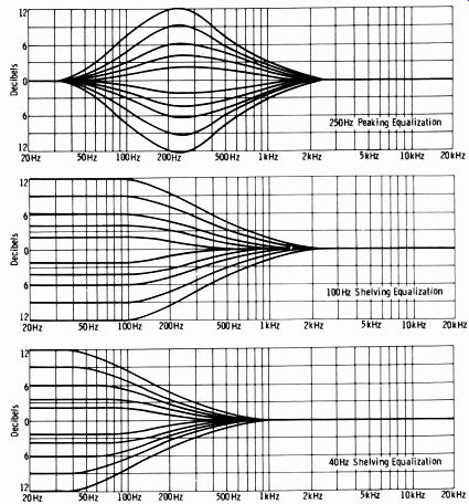
Fig. 6-20. Shelving and peaking curve of Electrodyne system (continued
on next page).
A block diagram of the Electrodyne system, which employs control modules of this type, is shown in Fig. 6-19. The Electrodyne Model 711L combines a low-noise microphone preamplifier; low- and high-frequency equalizers; and echo, cue, and program amplifiers into a single plug-in module.
Front-panel controls allow 12-dB boost and attenuation and reciprocal equalization curves for four low frequencies and four high frequencies.
Three of the high-frequency curves and two of the low-frequency curves can be selected as shelving or peaking curves (Fig. 6-20) . The low-frequency equalization points are selectable at 40, 100, 250, or 500 Hz. High-frequency equalization points are selectable at 1.5, 3, 5, or 10 kHz. The 1.5-kHz position is included to permit control over the critical range required for dialogue and vocal enhancement. The input selector lever ( a dual concentric switch) allows selections between microphone and line.
There are two positions for the line, one with a 20-dB pad to compensate for high-level input signals. A microphone-preamplifier gain knob is provided, allowing up to 50 dB of gain in the microphone position. Other positions provide 10, 20, 30, and 50 dB of attenuation.
Fig. 6-20. Shelving and peaking curves of Electrodyne system-cont.
The -50 dB position is desirable for handling the high signal levels of modern condenser microphones. This position allows signal levels as high as +18 dBm. A phase-reversal push-button switch is provided to give 180° phase shift to the incoming signal by switching between the inverting and noninverting inputs of an operational amplifier. One echo send pot and selector switch gives the operator a choice of echo send from ahead of the attenuator, ahead of the attenuator but after equalization, or after the attenuator and equalization.
NOTE: The design of equalization networks in general involves advanced study beyond the scope of this text. Equalizers are normally purchased from the manufacturer after applications and specifications are formed by the user. However, for those readers interested in all types of equalizer design, the following text is recommended:
Howard M. Tremaine: Audio Cyclopedia (Indianapolis: Howard W. Sams & Co., Inc., 1969).
6-5. THE CONTROL CONSOLE
The operations console may be quite complex in terms of the number of circuits and control functions. However, modern centers are designed and installed to achieve an easily operated setup that allows as nearly fool proof switching as possible along with flexibility of functions. Briefly, the general requirements are as follows:
1. Amplifiers are needed for stepping up the minute electric energy produced by turntable pickups, tape heads, and microphones; these are termed preamplifiers. High-level amplifiers are then required to make up losses in such control circuits as the variable attenuators.
Isolation amplifiers are required to feed such points as monitoring speakers so that no interaction occurs on program and rehearsal or recording lines.
2. Switching and mixing arrangements on the control console allow selection of the proper program source and blending of individual inputs for desired program "balance."
3. Facilities are provided for auditioning or rehearsing a program to follow, or for recording on tape for use at a later time. These facilities must not "cross-talk" on the regular program line.
4. Inputs and outputs of amplifiers may be normaled through jack panels to allow rapid rerouting of the signal in case of trouble in any one amplifier or channel, or for flexibility in feeding signals to any desired point.
5. Incoming and outgoing lines may be normaled through jack panels to permit receiving or transmitting the signal in any desired path.
Fig. 6-21 illustrates one type of modern commercially built console.
This completely transistorized center employs 24 illuminated touch-control keys which allow a total of 45 inputs, replacing the more conventional switches and knobs spread across the control board. Eight large control knobs (faders or attenuators) are provided, one for each of eight mixing channels. A fully interlocked cue-intercom system is also incorporated.
Some control consoles employ self-contained amplifiers and power sup plies. Others provide only the mixing controls, switches, push buttons and VU meters, with all amplifiers and power supplies interconnected from rack-mounted units. In all cases, reel-to-reel and cartridge tape equipment as well as the turntables are external units from the control console.
Courtesy Gates Division Harris-Intertype Corp.

Fig. 6-21. Dual-channel console employing transistor circuitry.
Network centers and larger independent stations sometimes use a facility known as a producer's console in conjunction with the individual studio control board. This panel contains a talk-back ( intercom) , production timing facilities, and appropriate signaling lights.
In large installations, a master control room may be used as the central switching facility. Each individual studio control is linked to the master control room by audio cables, relay control cables, tally-light ( signaling) cables, and intercom lines. The audio cable connects the studio output terminals to master-switcher relay contacts; the relay-control cable connects push-button switches and supervisory lamps in the individual studio switcher (through turnkey switches in the master) to the appropriate dc control circuits. Any studio console can be fed to a given number of out going channels-the turnkey switches permit the master-control operator to assign control of any channel to any studio console. Push-button switches and lamps in the master switcher are connected to the control circuits of all relays, allowing switching to be performed either by the master operator or studio operator.
Fig. 6-22 is a block diagram of the CCA Executive 8-fader, dual-function control console for AM or fm use. The 8-fader arrangement provides for up to 19 inputs. Nine inputs are for microphones, two for turntables, five for high-level lines switchable to two faders, and three for tape lines. Any single channel can be switched to the audition or program channel. Output lines are: program (1) , muted speaker (4) , intercom (5) , headphones (2), low-level production channel (1), and high-level (+18 dBm) production channel (1).
Three-position selector switches for the microphone and tape channels are mounted immediately above their corresponding attenuators. The channel 6 position is normally used for the control-room microphone. The turn table, tape, and remote-line faders contain a cue provision as described earlier in this Section.
The two remote (or network) faders have five high-level inputs avail able which can be switched to either of the two channels. It is impossible for the same input to be connected to both faders simultaneously; thus segueing" ( fading out one source while fading in the next source) between the two channels can be accomplished. When a remote-line input selector switch is in the center position, the program is fed back to that remote channel for cue or public-address amplifier feed at the remote pickup point.
The console monitor amplifier has facilities to select the program, audition (production), or external lines as a driving source. It also has facilities to drive the normal program or production lines. Thus it can serve as an emergency program line amplifier or a production line amplifier and simultaneously drive four speakers. The VU meter can be switched to the program line, the production line, or an external source.
Speaker Muting Circuitry
Whenever a microphone is turned on, the monitoring speaker in the same studio must be cut off simultaneously to avoid acoustical feedback.
This is accomplished by a control circuit which is tied through a set of contacts on the microphone switch and which operates a muting relay for the studio speaker. The speaker is thereby disconnected, and a resistor of equivalent impedance is placed across the monitor bus to provide the same termination. If this is not done, other speakers connected to the same monitor bus would exhibit varying sound levels as speakers were turned off and on.
While some speaker muting arrangements employ only relay contacts actuated from the microphone key, others, such as the one in the CCA Executive described above, incorporate transistor switches for the relays.
Fig. 6-23 illustrates the basic action of a two-studio system for purposes of discussion.
When the line-voltage ac is applied to the console, the +24-volt power supply is on, and all transistors (Q1 and Q2 in Fig. 6-23) are fully con ducting due to the base current through the 22K resistors. Therefore, the associated relays are energized, the monitor speakers are on, and the on-air lights are off. In Fig. 6-23, it is assumed that a microphone is turned on in Studio A. When a microphone key is dosed, the base of the corresponding transistor is shorted to ground, turning that transistor off and de-energizing the associated relay. This turns the on-air light on and mutes the monitor speaker by opening the high side of the circuit and substituting the back load resistor (R1 in this example) for the former speaker load resistance.
Thus the signal level on the monitor bus is maintained the same in other studios whether another studio monitor speaker is on or off.
With the transistor arrangement, there is virtually no "click" in the system as muting is accomplished, since there is a total of only about 1 mA that turns the relays on and off. Diodes across the relays are used to damp the system against counter emf's from the relay coils.

Fig. 6-22. Simplified diagram of CAA Executive 8-fader, dual-function, monaural
console.
Talk-Back System
The CCA console previously described is designed to provide front-panel talk-back to auxiliary channels 9 and 10. From Fig. 6-24, it can be seen that there is a transistor which is normally off. Turning the talk-back switch to studio A, B, C, or remote turns the transistor on by applying for ward bias to its base. This operates the talk-back relay. The talk-back relay reverses the cue bus so that the front-panel speaker serves as a microphone.
The output of this speaker goes through the talk-back switch, then the talk-back relay, then the cue amplifier, back again through the talk-back relay, then to the talk-back keys front-panel switch, and then to the appropriate studio speaker selected by the talk-back key. It should be noted that the monitor amplifier normally feeds the program channel to the auxiliary lines when the switches are in the center position.

Fig. 6-23. Speaker muting and on-air light arrangement.

Fig. 6-24. Talk-back board for CCA consoles.
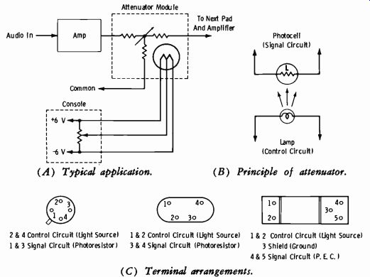
Fig. 6-25. Light-controlled attenuators. (A) Typical application. (B) Principle
of attenuator. (C) Terminal arrangements.
(A) FET as voltage variable attenuator.
(B) Typical FET switch circuit.

Fig. 6-26. Attenuators using FETs.
Electronic Attenuators and Switches
It now remains to become familiar with the latest type of electronic con sole gain controls; when these controls are used, audio itself is not brought into the control console except for VU-meter or monitoring purposes. In Fig. 6-25A, the light-controlled attenuator and light source are in one module which is placed in the audio circuitry. The control potentiometer is in the audio control console, which may be at some distance from the audio racks. Note in this case that the slider arm rotates between plus and minus voltages so that the constant impedance of the attenuator is maintained just as in mechanical faders.
Fig. 6-25B illustrates the basic principle of these controls. The cells are normally of the cadmium-sulfide type, and the intensity of the light or lights (located adjacent to the cell) changes the cell resistance, thereby affecting the gain of the audio path in which the cell is placed. This provides a noise-free control over a wide dynamic range without transients or contact chatter. The resistance decreases as the lamp intensity increases.
A current-limiting resistor may be found in series with the lamp, or a transistor constant-current source may be used. The control current is then linear with voltage over a stated range. Fig. 6-25C shows typical terminal arrangements.
The cell resistance at maximum light intensity may vary between about 50 and 150 ohms. The dark resistance may be as high as 100 megohms or more depending on type. A reaction time of 5 to 20 milliseconds is typical.
A defective unit is indicated by an open circuit between the control-circuit (lamp) terminals. Normal resistance at the lamp terminals as-14V checked with an ohmmeter is around 100 to 200 ohms, depending on the voltage rating of the lamp.

Fig. 6-27. Microphone preamplifier circuits. (A) Input stage. (B) Second
stage.
Fig. 6-26A illustrates another type of electronic attenuator, in which an FET is employed as a voltage-variable resistance. In this application, the drain-source voltage is biased below pinch-off. The series resistance is about 101° ohms when the gate is at maximum negative voltage, decreasing linearly to about 240 ohms with the gate at ground potential.
Fig. 6-26B shows a typical FET circuit used for audio switching in place of relay or key contacts. When the control voltage on the base of Q2 is zero, or low, Q2 is off and forms an open switch. Transistor Q1 is turned fully on, presenting a series impedance of about 240 ohms. When the control voltage on the Q2 base goes toward 1 volt (high) , Q2 saturates, forming a closed switch to apply-12 volts to the gate of Q1, turning the FET off. In this condition, the series resistance presented to the signal is about 101° ohms. Switches using FETs lend themselves readily to the logic portions of automation systems.
6-6. MICROPHONE PREAMPLIFIERS
A common microphone input circuit for broadcast application is shown in Fig. 6-27A. Broadcast microphones are always of low impedance, so the first requirement (low source resistance) for a low noise factor is met.
Second, the microphone normally has fairly long cables, so a transformer input is used to minimize hum and other extraneous pickup.
The primary of T1 is balanced to eliminate hum and noise pickup. The secondary is operated unloaded, which is conventional for low-impedance microphones. Note that the base of Q1 is series-fed from the secondary of T1; this is the type of feed often used in solid-state broadcast applications.
This technique minimizes any tendency toward load change with signal variation and results in maximum input gain (maximum transducer gain) from T1. The network R1-C1 across T1 is used to roll off frequencies above the audio passband; therefore, it is sometimes stated that the network provides high-frequency stabilization of the circuit.
Since VCE and the emitter current must be kept very low for a low noise factor, high values of RL (R4) and RE (R5-R6) are invariably found in the first stage of a preamplifier.
Now we will go through the dc analysis (operating point) for this stage.
Voltage divider R2-R3 provides about-2.2 volts to the base of Q1. Since the 2N422 is a germanium transistor, the emitter voltage will be about-2 volts. So the emitter current is 2/5.2K = 0.38 mA (approx) .
Assuming the collector current is the same as the emitter current, the collector voltage is
-[14- (0.38) (20) ) =-6.4 volts, so VcE _-6.4
-(-2) =-4.4 volts.
If you ignore negative feedback and the input impedance of the following stage, what voltage gain would you expect?
rte
0.3 + 100 = 168 and RL 20000 A° 120 (approx) rt,.- 168
Fig. 6-27B shows a typical second stage into which the circuit of Fig. 6-27A might be coupled. Since the emitter current of this second stage is 6.2/3.6K= 1.7 mA:
rt = i + 4= 19 (approx)
and
= (hre)(rtr.) = (40)(19) =750ohms (approx)
Now the effective RL of the first stage is 20K in parallel with 750 ohms, or about 720 ohms. Therefore the actual Av of the first stage (still ignoring any negative feedback) is:
RI, 720 Av
_ rt.,. 168-
4.3
In practice, negative feedback (which is usually applied by an arrangement similar to that in Fig. 6-27A) can bring the voltage gain down to unity or less (depending on the type of feedback).
This analysis has been made to emphasize a point: The first stage of a preamplifier is usually operating at a very low gain, sometimes an actual voltage loss, in the interest of maximum fidelity and low inherent noise.
A slightly different approach is taken in the RCA BA-72A preamplifier.
As shown by the simplified schematic of Fig. 6-28, this preamplifier consists of an unloaded input transformer (T101), a two-stage negative-feed back amplifier (Q1 and Q2) , a two-stage output amplifier (Q3 and Q4) , and an output transformer (T102). The Q1 collector load (R5) is 10K, the Q2 collector load (R13) is 2K, and the bypassed emitter resistor of Q2 (R14) is 200 ohms.
The high side of the input-transformer secondary is connected directly to the base of transistor Q1. This transistor operates in a common-emitter circuit with its collector connected to the base of Q2 through capacitor C6.
Transistor Q2 also operates in a common-emitter circuit. The emitter resistor of Q2 is completely bypassed by capacitor C8, making the input impedance of Q2 very low. The low input impedance causes a larger signal current in the base of Q2, which results in a higher signal voltage developed across R13, the collector load resistor.
Negative feedback current passes from the collector of Q2 to the emitter circuit of Q1 through C9 and R9. Capacitor C5 bridges R9 to improve the signal response at high frequencies. The feedback is used mainly for stabilizing the gain and reducing distortion. As shipped from the factory, the 46-dB terminals are not strapped, and the gain of the preamplifier is 40 dB.
If 46-dB gain is desired, a strap is provided which shunts R4 across R7, thereby reducing the inverse feedback voltage developed in the emitter circuit of Q1.

Fig. 6-28
The voltage developed across R13 is direct-coupled to the base of Q3, which operates as an emitter follower. The emitter of Q3 is coupled by C12 to the primary winding of the output transformer, T102. The voltage developed across R15 is applied through C10 to the base of Q4. The collector output of Q4 is direct-coupled to the emitter of Q3, where it then passes through C12 to the output transformer. In the Q3-Q4 circuit, a current increase in Q3 causes a decrease in Q4. In effect, Q4 is a variable emitter load for emitter follower Q3, which results in increased current in output transformer T102.
Note that in the description of the negative feedback circuit above, it was stated that C5 (620 pF) across R9 (6190 ohms) improves the high-frequency response. Capacitor C9 (15 µF) has no frequency discrimination. Since this is negative feedback, as the frequency is increased with decreased reactance of C5, more inverse feedback is provided, decreasing the high-frequency gain while reducing distortion. The highest frequency of concern in the audio passband is 20 kHz. But a rapid roll-off above this frequency must not occur since high harmonic distortion results in distortion of the fundamental frequencies. The reactance of C5 at the second harmonic of 20 kHz (40 kHz) is about 6200 ohms, or approximately equal to the resistive value of R9 (6190 ohms) . In this manner, excellent frequency response at very low harmonic distortion is obtained. For the same reason (obtaining high-frequency stabilization), a 430-pF capacitor is shunted across the input transformer secondary (not shown on simplified schematic). Without such stabilization, supersonic oscillations can occur, and this would result in high total harmonic distortion.
(A) Balanced input. (B) Unbalanced input.
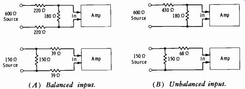
Fig. 6-29. Matching pads for amplifier driven by a preceding amplifier.
6-7. AMPLIFIER INPUT LOADING
The input transformer of a professional audio amplifier generally provides for a source impedance of either 150 or 600 ohms. It may be adjusted for either impedance by transformer taps. In actuality, for an unloaded input transformer, the input impedance is higher than the source impedance for all frequencies from 20 to 20,000 Hz. An amplifier can never be fed from the output transformer of a previous amplifier (such as using the amplifier as a booster) without resistive loading of the input to provide a constant impedance across the passband. The unloaded input transformer is used only when driven by a microphone or low-impedance source such as a phono pickup.
Minimum-loss (6 dB) matching pads for this purpose are shown in Fig. 6-29. Additional pads may be required to reduce the level at the amplifier input terminals to its specified maximum value.
6-8. TURNTABLE PREAMPLIFIERS
In practice, it is impossible to consider the stylus, pickup head, and preamplifier separately since each depends on the other. Even recording characteristics themselves must be included in the overall discussion. There are two basic methods of recording, the constant-velocity and the constant-amplitude methods.
Constant-Velocity Recording
Constant velocity refers to the maximum transverse velocity of the stylus tip at the mean axis. Since this is held constant as the frequency changes, the peak amplitude is inversely proportional to the frequency (Fig. 6-30A). The maximum slope of the curve is the same for all frequencies.
(A) Constant-velocity recording. (B) Constant-amplitude recording.

Fig. 6-30. Two basic methods of recording.
This method of recording is not suitable over a wide frequency range. For example, over a range of 8 octaves (each octave doubles the frequency) the ratio of maximum to minimum amplitudes is 256 to 1. This results in an impractical variation in peak amplitudes of the recorded grooves.
Constant-Amplitude Recording
The peak amplitude is held constant (for constant power output) as the frequency changes; therefore, the maximum slope is proportional to the frequency (Fig. 6-30B) . This method is satisfactory for low frequencies but is not suitable for large amplitudes at the highest frequencies.
This is due to excessive transverse velocity of the needle tip, which produces distortion in both recording and reproduction.
Combination Recording
Constant-amplitude recording is optimum for low frequencies; constant-velocity recording is quite satisfactory over a limited range including the medium and high frequencies. Therefore, practical recording systems em ploy an approximation to constant-amplitude recording at low frequencies and an approximation to constant-velocity recording for the medium- and high-frequency range. The crossover from constant amplitude to constant velocity normally occurs near 500 Hz. Any difference in the crossover frequency requires a different playback equalization for a flat frequency response.
Since the maximum slope of the displacement curve in the constant-amplitude mode is proportional to the frequency (Fig. 6-30B) , an increased voltage is obtained with an increase in frequency. The voltage increases 6 dB per octave. The "knee" of the crossover region is rounded off; that is, there is no sharp demarcation between the constant-amplitude and constant-velocity characteristics. The recording then enters the constant-velocity region and high-frequency preemphasis.

Fig. 6-31. EIA standard lateral disc-recording characteristic.

Table 6-6. Lateral Disc Characteristics (EIA, NAB, and RIAA)
In practice, both the low- and high-frequency regions undergo certain equalization procedures which modify the recording characteristics just described. For standardization, the slope of the curve in decibels per octave is normally stated as a time constant. For example, a simple RC network comprising a tone control is standardized by the RC time constant. Fig. 6-31 illustrates the EIA standard lateral disc-recording characteristic. Table 6-6 tabulates the recording and complementary playback curves. This characteristic has been adopted by NAB and RIAA.
The standard recording characteristic is specified as the algebraic sum of the ordinates (expressed in decibels) of three individual curves that con form to the admittances of the following three networks:
1. A parallel LR network having a time constant of 3180 µs.
2. A series RC network having a time constant of 318 µs.
3. A parallel RC network having a time constant of 75 µs.
Note from the curve of Fig. 6-31 that these three time constants specify the equalization of the frequencies up to the crossover frequency of 500 Hz, the rolloff of the crossover point itself, and the high-frequency pre-emphasis.


Fig. 6-32. Preamplifier for pickup.
The overall combination of the stylus, pickup head, arm, and preamplifier equalizer must provide the proper complementary reproduction characteristic given in Table 6-6. Then the overall response will be "flat."
Circuit Analysis of Typical Phonograph Preamplifier
Fig. 6-32 shows a typical preamplifier for a magnetic phonograph pickup or tape head. This circuit was chosen purposely to explain how one would go about analysis of the dc operating point. Note that the base of Q1 is biased from a current that is directly proportional to the emitter current of Q2. This connection stabilizes voltage and current bias points for changes in operating temperature and transistor hFE.
This circuit would be difficult to analyze for dc voltage operating point except for the basic rule of thumb that class-A amplifiers have a collector voltage somewhere near one-half the collector supply voltage. (This rule applies to the second and following stages of a preamplifier, never to the first stage.) If we start with the assumption of -11 volts at the Q2 collector, we can see how close we would come to the actual voltage readings shown, as follows:
Since this is a class-A amplifier, assume the Q2 collector voltage is one half the collector supply voltage, or -11 volts. Then for Q2:
IE 10K=1.1mA IE = 1.1 mA (approx) VE=(-1.1mA) (2700 ohms) =-3.0 V VB=-3.OV+(-0.2V)
=-3.2 V (2N508 is germanium) Now, for Q 1:
VE =-3.2 V
Drop across RLR =-22 V- (-3.2 V) = 18.8 V
In=18.8/20K=0.94mA
IE = 0.94 mA ( approx ) VE = (-0.94 mA) (1600 ohms) =-1.5 V VB=-1.5 + (-0.2) =-1.7 V
Note also the similarity of this circuit to those of Fig. 6-27A and Fig. 6-27B combined. The second stage has a relatively low input impedance.
Response-curve equalization is sometimes located in the negative-feed back circuit, as in Fig. 6-32. Fig. 6-33 shows a typical feedback network for RIAA/NAB playback characteristics. Note that the capacitors across the resistors provide more feedback at high frequencies than at lower frequencies. Since this is a degenerative circuit, high-frequency response is reduced to provide the proper playback response. This method eliminates the need to load a magnetic cartridge with the proper resistance for high-frequency compensation. Just as in the case of a microphone, a magnetic phonograph pickup is best operated into a relatively high-impedance circuit with proper equalization following the input.
The output stage of a broadcast preamplifier normally feeds a 150-ohm or 600-ohm fader. Fig. 6-34A shows a typical emitter-follower output circuit. To review the analysis of this stage, assume a 600-ohm fader, a 720-ohm source resistance, and a /3 of 50. Then: 720 = 14 ohms (approx) 50 + 1 and:
R2 = 600- 14 = 586 ohms ( nearest EIA value = 560 ohms)
Fig. 6-34B shows the typical output stage when a transformer is used.
The negative feedback provided by Rt reduces the output impedance as well as the input impedance. The output-transformer primary is always loaded with a fixed resistor to insure a fixed load on the collector circuit.

Fig. 6-33. RIAA/NAB feedback network.
6-9. AUDIO SYSTEM TECHNOLOGY
(A) Emitter follower.
(B) Use of transformer.

Fig. 6-34. Attenuator coupling.
This section will describe the overall audio system, including program (line) and monitor amplifiers and the fundamentals of automatic audio signal processing systems. The simple installation of Fig. 6-35 will serve for basic discussion. Circuit impedances of 150 ohms are typical up to the line feed of 600 ohms, but all the impedances could be 600 ohms. Conversely, many lines now have 150-ohm impedances, and all circuits in the studio might be 150 ohms.
A typical level at the microphone input is -50 dBm. The gain of the preamplifier is 40 dB, so the output into the mixing circuitry is -10 dBm.
Typical operating mixer loss is 18 dB, giving-28 dBm at the mixer output. Since the maximum input level to most line amplifiers is around -32 to -35 dBm, a 10-dB pad loads the mixer output to provide a line-amplifier input level of -38 dBm. In this example, the line amplifier is adjusted to provide +18 dBm into the master-gain attenuator. A typical loss setting here is 10 dB, providing +8 dBm to the line-isolation pad. The VU-meter multiplier is set so that a level of +8 VU at this place in the system gives 0 deflection on the meter. (At this point, it should be emphasized that the reader must have a good working grasp of VU, dB, and dBm relationships. Review Section 2-10, Section 2) .
Typical Program (Line) Amplifier
A simplified schematic of the RCA BA-43 program amplifier is shown in Fig. 6-36. This unit consists of an input transformer and a two-stage feedback preamplifier coupled through an emitter follower to a four-stage output amplifier.

Fig. 6-35. Typical broadcast audio circuit.

Fig. 6-36
The input signal is applied to the primary of transformer T1. The transformer has a split primary; the two halves are connected in series for 600-ohm sources and in parallel for 150-ohm sources. The secondary of the transformer is unloaded. To obtain a 600- or 150-ohm input impedance, a 600- or 150-ohm resistor must be connected across the primary. The signal from the secondary of Ti is applied through capacitor C2 to the base of Q1. The amplified signal from the collector of Q1 is applied to the base of Q2 and is again amplified. The signal from the collector of Q2 is applied through resistor R9 to the base of emitter follower Q3. Negative feedback current from Q3 to Q1 passes through resistor R7. The output of the pre amplifier passes through C5 to gain control R8 and then to terminal 9 of connector P1.
The operation of the output-amplifier portion is as follows: The input signal goes from terminal 1 of connector P1 to the base of Q4, is amplified, and is coupled to the base of Q5 through capacitor C7. The signal is amplified by Q5 and Q6, and the output from the collector of Q6 is applied to the bases of Q8 and Q9 which operate as a complementary-symmetry output stage. The output from the emitters of Q8 and Q9 is applied through C18 to output transformer T2. A dc (only) feedback loop exists through R17 between the Q6 emitter and the Q5 base. A second feedback loop in the output amplifier is formed by R23 and C12 between the output and the Q5 emitter. The result is a frequency response which is better than ±1 dB from 20 to 20,000 Hz at the maximum output level of +30 dBm.
At this output level, the output noise level is less than -43 dBm, giving a signal-to-noise ratio of 73 dB, at a total harmonic distortion of 0.5 percent maximum.
Automatic Level-Control Systems
The trend in modern broadcast techniques is toward the use of automatic level-control equipment. Manual gain riding, a burdensome task at best, has the disadvantage of inhibiting the station from operating at its highest potential power. Every system is limited to a level which results in 100 percent modulation of the transmitter. Since maximum use must be made of the authorized power, and since highest signal-to-noise ratio is obtained for high degrees of modulation, it is desirable to maintain the average level of modulation as high as practicable. In addition, complete automation re quires the use of automatic level riding to maintain high modulation levels without exceeding FCC modulation limits.
For automatic systems, some form of agc (automatic gain control) amplifier is normally employed at the studio. This amplifier has the ability to hold a relatively constant average output level over a wide range of input levels; this ability far exceeds that which can be obtained with manual gain riding. However, since this gain-control function must be performed in an inaudible manner, it is designed to be relatively slow acting when compared to the capability of electronic circuitry to act in fractions of a microsecond.
These relatively slow attack and release times are not sufficient to prevent fast-acting signal peaks from over-modulating the transmitter. Therefore a limiter amplifier to control the faster-acting signal peaks is normally used at the transmitter.
(A) Limiter amplifier. (B) Agc amplifier.

Fig. 6-37. Audio level-control devices.
Fig. 6-37A shows a block diagram of the fundamental audio amplitude limiter. Fig. 6-37B shows a block diagram of the fundamental agc system.
The differences between these circuits will be discussed in the following paragraphs.
Limiter (or compressor) amplifiers normally employ only the closed-loop arrangement of Fig. 6-37A. This loop is degenerative, acting to reduce the gain as the input signal rises above a given level. For instance, an in put-signal increase of 10 dB might result in an increase at the output of only 1 dB. The gain reduction (in this example 9 dB) is the amount the signal has been limited or compressed.
In addition to gain reduction on high signals, the agc amplifier (Fig. 6-37B) allows a gain expansion over a limited range of lower-level signals.
This combination of expansion and limiting, using both the open-loop and closed-loop control, maintains high uniform average levels without over-modulation and (ideally) without raising the noise level during dead sound intervals.
When agc is used in stereo applications, an additional factor is involved.
It is important to maintain the original amplitude difference between channels so that maximum separation effect is obtained. Using a separate agc amplifier in each channel results in equal left and right volume, and some of the stereo positioning is lost. This problem is solved by tying the agc amplifiers together so that both have the same dc gain-control signal. This maintains relative gains, and the amplitude difference is preserved.
The most common types of gain-controlling devices are those that have variable amplification, those that exhibit a variable impedance, or those that exhibit both methods combined. For example, amplification can be made quite dependent on base bias; this bias can be supplied by the dc gain-control signal.
The power rectifier in the blocks of Fig. 6-37 is typified by the circuit of Fig. 6-38. It is a filtered dc amplifier driven from the signal-rectifier diode. In some cases, only the base-emitter junction is used as the rectifier at the expense of the power gain.

Fig. 6-38. Power rectifier circuit diagram.
Fig. 6-39A shows an example of amplification dependent on base bias.
The transistor, biased in the active region, has its base voltage modified by the agc voltage from the power rectifier. Note from Fig. 6-39B that the slope of the curve (ratio of change in collector current to change in base-emitter voltage) is affected. As the signal increases, a larger negative agc voltage is applied to drive the transistor toward cutoff. The maximum gain reduction available in this type of circuit is about 15 dB if serious non linear distortion is to be avoided.
(A) Circuit diagram. (B) Variation of gain.

Fig. 6-39. Base-bias control of gain.
In Fig. 6-40 is an example of variable impedance in parallel with the signal path. When the current through a diode increases, the diode resistance decreases, and vice versa. The input current divides between the amplifier input and the diode resistance, RD. When the signal is increased, the agc voltage increases and RD decreases, lowering the overall stage gain.
With this type of circuit, the signal source must have a high resistance (Rs), and the amplifier input impedance must be high also.
(A) Circuit diagram. (B) Diode resistance.

Fig. 6-40. Variable-impedance gain control.
Fig. 6-41 shows a two-terminal shunt arrangement. If a large agc voltage is developed (large signal) , Q2 will have maximum base current and will saturate. Capacitor C2 is then returned to ground and provides a short circuit to the signal. As less agc is developed, Q2 assumes a higher shunt impedance (because its base current is decreased) , and the gain is increased.
Most of the agc action occurs in the region near Q2 saturation, where the slope of the output characteristic is changing most rapidly.
The RCA BA-45 AGC Unit
The RCA BA-45 agc unit contains expansion and compression circuits located on separate etched wiring boards. The BA-45 is designed for use with the BA-43 program amplifier and provides either expansion or compression, or both, by means of independent switches mounted behind the front panel. With both expansion and compression disabled, the BA-43 program amplifier will perform as a normal program amplifier with approximately 10 dB less gain than with a BA-43 operating alone. Refer to Figs. 6-42 and 6-43 for the following description.
(A) Circuit diagram. (B) Transistor operation.

Fig. 6-41. Variable impedance with transistor.

Fig. 6-42

Fig. 6-43
The expansion circuitry consists of an emitter follower, audio amplifiers, a full-wave threshold gate, a pulse amplifier, an emitter follower, and an average detector. The audio signal to the expansion circuitry is applied from the preamplifier section of the BA-43 program amplifier through terminals 9 and 11 of connector P1 and disable/expansion switch S2 to the base of emitter follower Q6. The audio signal from the emitter of Q6 is applied to the base of Q7 and is further amplified by audio amplifiers Q7, Q8, and Q9. The outputs from the emitter and collector of Q9 are applied to a full-wave threshold gate consisting of X6, X7, and associated circuitry. This gate sets the threshold level for expansion. The resulting pulses from the full-wave threshold gate are applied to the base of pulse amplifier Q10 and then to the base of emitter follower Q11. The signal from the emitter of Q11 is applied to the average detector, X8 and R28.
This average detector provides a relatively slow attack and release time of Fig. 6-44. Input-output characteristics of BA-43 and BA-45 combination.
approximately 5 seconds, for 10 dB of expansion. The resultant dc signal is applied to the base of dc driver Q5. This driver controls the current through the incandescent-lamp section of the light-dependent resistor (LDR), RT1. A change in light intensity causes a corresponding change in the resistance section of RT1. Components R29, R57, and RT1 form a voltage divider which varies the audio signal level to the output-amplifier section of the BA-43 program amplifier. See Figs. 6-44 and 6-45.

Fig. 6-45. Gain characteristics of BA-43 and BA-45 combination.
The compression circuitry consists of a full-wave threshold gate, pulse amplifiers and a phase inverter, a full-wave detector, an emitter follower, and a peak detector. The compression circuitry shares the dc driver and the LDR with the expansion circuitry.
The audio input to the compression circuitry is applied from the output amplifier section of the BA-43 through terminal 7 of connector P1 and disable/compression switch S1 to the full-wave gate which consists of Xl, X2, and associated circuitry. This gate sets the threshold level for compression. The resulting pulses from the full-wave threshold gate are applied to pulse amplifiers Q1 and Q2. One output from the collector of Q2 is applied through C5 to the full-wave detector which consists of X3, X4, and associated circuitry. Another output from the collector of Q2 is inverted by Q3 and then applied through C6 to the full-wave detector. The resulting pulses are applied to the base of emitter follower Q4. The output from the Q4 emitter is applied to the peak detector which consists primarily of X5, C7A, and C7B. Components X5, C7A, C7B, and Q4 make up a fast charging circuit which provides the compression circuitry with a rapid attack time (15 milliseconds for 10 dB of compression) . When the audio signal drops below the compression threshold, X5 becomes an open circuit, and C7 then discharges through a higher impedance at the slower rate of 3 seconds for 10 dB of compression. The dc signal from the peak detector is applied to the base of emitter follower Q5. Transistor Q5 operates in the manner described above.

Fig. 6-46. Typical monitor-amplifier output transformer. (A) Parallel feed.
(B) Series feed.

Fig. 6-47. Matched-impedance feed of multiple speakers.
Monitor-Speaker Distribution
It is sometimes necessary to employ several speakers in a studio or other location, particularly where the area is large and the acoustics are influenced by the number of persons present. Fig. 6-46 shows a typical monitor output transformer with connections provided to meet a variety of applications.
Fig. 6-47 reviews the basic principles of matching multiple speakers to the monitor-line feed. Fig. 6-47A illustrates how two 16-ohm speakers may be connected in parallel to the 8-ohm monitor output terminals. Each speaker receives half the total power on the line. Fig. 6-47B shows two 8-ohm speakers connected in series to the 16-ohm monitor output terminals.
Again, each speaker receives half the total line power. Any combination may be used: two 4-ohm speakers could be placed in series to feed from the 8-ohm line; two 8-ohm speakers could be paralleled to feed from the 4-ohm line, etc.
Due to the relatively large amount of current required for a given power, low-impedance monitor lines (such as 4 to 16 ohms) are limited to a short length of run for a practical wire size. When monitor lines must be long, lines of 150- or 600-ohm impedance are generally used. Table 6-7 gives the pertinent values of wire size and maximum feed length for the various impedances.

Table 6-7. Maximum Length in Feet for Monitor Lines
For very long monitor runs such as might be encountered at field events and associated pa coverage, a constant-voltage line, generally of the 70-volt level, is usually used, as shown in Fig. 6-48. With this technique, various speakers may be switched on or off without substituting back-load resistors and with little effect on the volume from other speakers. Speakers are connected across the distribution line through transformers that reduce the audio line voltage to the desired speaker level.

Fig. 6-48. 70-volt speaker distribution line.
In actuality, the audio line voltage is strictly dependent on the output regulation characteristics of the monitor amplifier driving the line. Amplifiers which provide for a 70-volt line feed should have output regulation such that the audio voltage has a maximum variation of 1.5 dB from no load to full load. The full-load requirement must not exceed the amplifier capability.
Reviewing Fig. 6-46, note that the 600-ohm line feed and the 70-volt line feed are identical. This really means that the transformer illustrated is probably associated with a 10-watt monitor amplifier. Thus with 8 watts feeding 600 ohms, the audio voltage is about 70 volts. For 50 watts of audio power on the line, a 100-ohm output would be used. In practice, monitor amplifiers designed for 70-volt line feeds have the 70-volt tap designated on the output transformer so that no computation is necessary regardless of the power rating of the amplifier. In practice, the actual audio line voltage varies with the signal. The 70-volt designation simply means the output voltage for maximum power.
In multiple speaker installations, it is usually desirable to be able to control the volume of one or more of the individual speakers. Fig. 6-49A shows the normal method used for a 70-volt line. When the monitor audio is distributed at voice-coil impedances, the T pad (Fig. 6-49B) or L pad (Fig. 6-49C) may be used. The L pad presents a constant impedance in one direction only (the side toward the monitor line) .
(A) Tapped secondary. (B) T-pad control. (C) L-pad control.

Fig. 6-49. Control of volume of individual speakers.
Proper Grounding Techniques
Hum, noise, and cross talk in any given installation are highly dependent on the technique of grounding. Every rack of equipment should have the grounds heavily strapped to a common point on that rack, and all rack grounds should be connected with good copper strapping to a common system ground point.
Fig. 6-50 gives the basic principle of microphone wiring. The cable from the studio wall outlet to the microphone should be a shielded twisted pair with flexible rubber covering for ease of handling and minimum shock noise if the cable needs any movement during use. The shield wire must not contact ground at any point in the system until it encounters the first preamplifier in the control room.
In extremely large installations, two grounding systems are employed: an equipment chassis ground, and a separate signal ground. In this case, the microphone-circuit ground is carried to the separate signal ground.
A cable with three wires plus a shield is often used for microphone circuits. In this event, the shield and third wire are tied together to form a more reliable ground connection over long periods of possible rough handling in service.
For jack fields, the sleeve or frame should preferably be mounted on a copper strap carried across the width of the panel, to provide convenient connection to the system or signal ground.
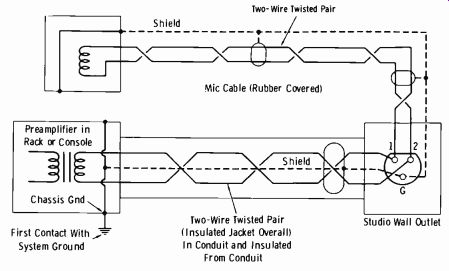
Fig. 6-50. Proper grounding of a microphone circuit.
In system or rack wiring, careful attention should be given the routing of cable forms carrying widely different signal levels. Three level specifications should be used, as follows:
1. Low level: Below-10 dBm, such as microphone circuitry
2. Intermediate level: -10 dBm to +20 dBm, such as rack amplifiers, boosters, and special effects (echo, reverberation, etc.)
3. High level: above +20 dBm, such as monitor lines, where +40 dBm is common
Cable forms of these three levels should be separated from each other by a distance of at least 2 inches.
All balanced mixing circuits employ center taps on the potentiometers, which may or may not need grounding. A test for best signal-to-noise (and signal-to-hum) ratio will determine whether this is necessary.
EXERCISES
Q6-1. Assume a balanced 600-ohm line carries a signal level of +10 dBm.
This must feed an amplifier of 150-ohm balanced input impedance.
The specified maximum input level for this amplifier is -22 dBm.
Design the proper pad for this purpose.
Q6-2. What is the minimum insertion loss of a mixer potentiometer?
Q6-3. What is the minimum insertion loss of a ladder attenuator?
Q6-4. What is the minimum insertion loss of a:
(A) T attenuator. (B) H attenuator.
Q6-5. A preamplifier with a fixed gain of 40 dB is rated as having a noise level of-80 dBm referred to the output. What is the minimum input level required to maintain a signal-to-noise (s/n) ratio of 60 dB?
Q6-6. If the preamplifier of Q6-5 is rated at a maximum output level of +18 dBm, what is (A) the maximum input level (B) the s/n ratio at maximum input level?
Q6-7. It is necessary to bridge a 600-ohm line carrying a 0-dBm level. An amplifier available for the bridging circuit has a balanced 600-ohm input and must have an input level of -25 dBm to obtain the required output. How could this bridging be done with resistors?
Q6-8. Assume you must build a four-microphone low-level T mixer to include a master gain control. The microphones are 150 ohms. What is:
(A) The value of R (see Fig. 6-14). (B) The input level to the amplifier following the master gain control if the microphones give a-60-dBm output?
Q6-9. What s/n ratio would you expect from the amplifier of Q6-5 in the circuit of Q6-8?
Q6-10. Assume four 4-ohm speakers are connected in series across an 8-watt, 16-ohm monitor line. How many watts does each speaker receive?