26. The z-transform
Whereas it was possible to design effective FIR filters with relatively simple theory, the IIR filter family are too complicated for that. The z-transform is particularly appropriate for IIR digital filter design because it permits a rapid graphic assessment of the characteristics of a proposed filter. This graphic nature of the z-plane also lends itself to explanation so that an understanding of filter concepts can be obtained without their becoming obscured by mathematics.
Digital filters rely heavily on delaying sample values by one or more sample periods. One tremendous advantage of the z-transform is that a delay which is difficult to handle in time-domain expressions corresponds to a multiplication in the z-domain. This means that the transfer function of a circuit in the z-domain can often be written down by referring to the block diagram, which is why a register causing a sample delay is usually described by z-1. The circuit configuration of FIG. 60(c) is repeated in FIG. 63(a).
For simplicity in calculation, the two coefficients have been set to 0.5. The impulse response of this circuit will be found first, followed by the characteristics of the circuit in the z-plane which will immediately give the frequency and phase response.
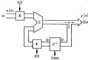
FIG. 63 (a) A digital filter which simulates an RC network. In this example
the coefficients are both 0.5.
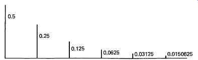
FIG. 63 (b) The response of (a) to a single unity-value sample. The initial
output of 0.5 is due to the input coefficient. Subsequent outputs are always
0.5 of the previous sample, owing to the recursive path through the latch.
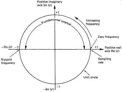
FIG. 63 (c) The z-plane showing real and imaginary axes. Frequency increases
anticlockwise from Re(z) = +1 to the Nyquist limit at Re(z) = -1, returning
to Re(z) = +1 at the sampling rate. The origin of aliasing is clear.
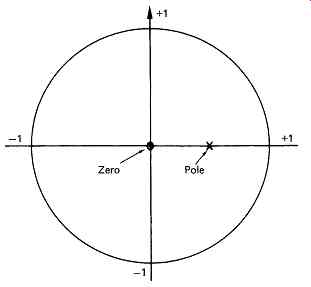
FIG. 63 (d) The z-plane is used by inserting poles and zeros.
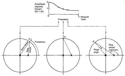
FIG. 63 (e) Some examples of response of the circuit (a) using the z-plane.
The zero vector is divided by the pole vector to obtain the amplitude response,
and the phase response is the difference between the arguments of the two vectors.
The impulse response can be found graphically by supplying a series of samples as input which are all zero except for one which has unity value.
This has been done in the figure, where it will be seen that once the unity sample has entered, the output y will always be one half the previous output, resulting in an exponential decay.
Where there is a continuous input to the circuit, the output will be one half the previous output y plus one half the current input x. The output then becomes the convolution of the input and the impulse response.
It is possible to express the operation of the circuit mathematically.
Time is discrete, and is measured in sample periods, so the time can be expressed by the number of the sample n. Accordingly the input at time n will be called x[n] and the corresponding output will be called y[n]. The previous output is called yn-1. It is then possible to write:
y[n] = 0.5 x[n] + 0.5 y[n-1]
This is called a recurrence relationship, because if it is repeated for all values of n, a convolution results. The relationship can be transformed into an expression in z, referring to FIG. 63(b):
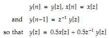
As with any system the transfer function is the ratio of the output to the input. Thus:
The term in the numerator would make the transfer function zero when it became zero, whereas the terms in the denominator would make the transfer function infinite if they were to become zero. These result in poles.
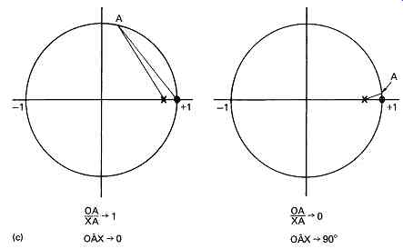
Poles and zeros are plotted on a z-plane diagram. The basics of the z-plane are shown in FIG. 63(c). There are two axes at right angles, the real axis Re(z) and the imaginary axis Im(z). Upon this plane is drawn a circle of unit radius whose centre is at the intersection of the axes.
Frequency increases anticlockwise around this circle from 0Hz at Re(z) = +1 to the Nyquist limit frequency at Re(z) = -1. Negative frequency increases clockwise around the circle reaching the negative Nyquist limit at Re(z) = -1. Essentially the circle on the z-plane is produced by taking the graph of a Fourier spectrum and wrapping it round a cylinder. The repeated spectral components at multiples of the sampling frequency in the Fourier domain simply overlap the fundamental interval when rolled up in this way, and so it is an ideal method for displaying the response of a sampled system, since only the response in the fundamental interval is of interest. FIG. 63(d) shows that the z-plane diagram is used by inserting poles (X) and zeros (0).
In equation (2), H[z] can be made zero only if z is zero; therefore a zero is placed on the diagram at z = 0. H[z] becomes infinite if z is 0.5, because the denominator becomes zero. A pole (X) is placed on the diagram at Re(z) = 0.5. It will be recalled that 0.5 was the value of the coefficient used in the filter circuit being analyzed. The performance of the system can be analyzed for any frequency by drawing two vectors. The frequency in question is a fraction of the sampling rate and is expressed as an angle which is the same fraction of 360 degrees. A mark is made on the unit circle at that angle; a pole vector is drawn from the pole to the mark, and the zero vector is drawn from the zero to the mark.
The amplitude response at the chosen frequency is found by dividing the magnitude of the zero vector by the magnitude of the pole vector. A working approximation can be made by taking distances from the diagram with a ruler. The phase response at that frequency can be found by subtracting the argument of the pole vector from the argument of the zero vector, where the argument is the angle between the vector and the positive real z-axis. The phase response is clearly also the angle between the vectors. In FIG. 63(e) the resulting diagram has been shown for several frequencies, and this has been used to plot the frequency and phase response of the system. This is confirmation of the power of the z-transform, because it has given the results of a Fourier analysis directly from the block diagram of the filter with trivial calculation. There cannot be more zeros than poles in any realizable system, and the poles must remain within the unit circle or instability results.
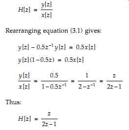
FIG. 64(a) shows a slightly different configuration which will be used to support the example of a high-pass filter. High-pass filters with a low cut-off frequency are used extensively in digital audio to remove DC components in sample streams which have arisen due to convertor drift.
Using the same terminology as the previous example:
u[n]= x[n] + Ku[n-1] so that in the z-domain:
u[z]= x[z] + Kz-1 u[z] (eqn. 3)
FIG. 64 (a) Configuration used as a high-pass filter to remove DC offsets
in audio samples. (b) The coefficient K determines the position of the pole
on the real axis. It would normally be very close to the zero.
(c) In the passband,
the closeness of the pole and zero means the vectors are almost the same
length, so the gain tends to unity and the phase shift is small (left). In
the stopband, the gain falls and the phase angle tends to 90°.
Also: y[n]= u[n]- u[n-1] So that in the z-domain:
y[z]= u[z]- z-1 u[z]= u[z](1-z1 ) Therefore:
y[z] uz
=1-z-1 (3.4) From equation (3) u[z]- Kz-1 u[z]= x[z] Therefore:
u[z](1-Kz-1 )= x[z] and u[z] x[z]
= 1 1-Kz-1 (eqn 5)
From equations (4) and ( eqn 5):
y[z] x[z]
= y[z] u[z]
_ u[z] x[z]
= 1-z 1-Kz-1
Since the numerator determines the position of the pole, this will be at z = 1, and the zero will be at z = K because this makes the denominator go to zero. FIG. 64(b) shows that if the pole is put close to the zero by making K almost unity, the filter will only attenuate very low frequencies.
At high frequencies, the ratio of the length of the pole vector to the zero vector will be almost unity, whereas at very low frequencies the ratio falls steeply becoming zero at DC. The phase characteristics can also be established. At high frequencies the pole and zero vectors will be almost parallel, so phase shift will be minimal. It is only in the area of the zero that the phase will change.
27. Bandpass filters
The low- and high-pass cases have been examined, and it has been seen that they can be realized with simple first-order filters. Bandpass circuits will now be discussed; these will generally involve higher-order configurations. Bandpass filters are used extensively for presence filters and their more complex relative the graphic equalizer, and are essentially filters which are tuned to respond to a certain band of frequencies more than others.
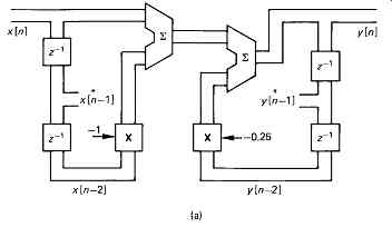
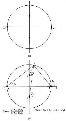
FIG. 65 (a) Simple bandpass filter combining lead and lag stages. Note that
two terms marked have zero coefficients, reducing the complexity of implementation.
(b) Bandpass filters are characterized by poles which are away from the real
axis. (c) With multiple poles and zeros, the computation of gain and phase
is a little more complicated.
FIG. 65(a) shows a bandpass filter, which is essentially a lead filter and a lag filter combined. The coefficients have been made simple for clarity; in fact two of them are set to zero. The adder now sums three terms, so the recurrence relationship is given by:
y[n]= x[n] - x[n-2] - 0.25y[n-2] Since in the z-transform x[n-1] = z-1 x[n], y[z]= x[z] - z-2 x[z] - 0.25z-2 y[z] H[z]= y[z] x[z]
= 1-z-2 1 + 0.25z-2
= z2 -1 z + 0.252
As before, the position of poles and zeros is determined by finding what values of z will cause the denominator or the numerator to become zero. This can be done by factorizing the terms. In the denominator the roots will be complex:
z2
-1 z2
+0.25
= (z+1)(z-1) (z+j0.5)(z-j0.5)
FIG. 65(b) illustrates that the poles have come off the real axis of the z-plane, and then appear as a complex conjugate pair, so that the diagram is essentially symmetrical about the real axis. There are also two zeros, at Re+1 and Re-1.
With more poles and zeros, the graphical method of determining the frequency response becomes more complicated. The procedure is to multiply together the lengths of all the zero vectors, and divide by the product of the lengths of all the pole vectors. The process is shown in FIG. 65(c). The frequency response shows an indistinct peak at half the Nyquist frequency. This is because the poles are some distance from the unit radius.
A more pronounced peak can be obtained by placing the poles closer to unit radius. In contrast to the previous examples, which have accepted a particular configuration and predicted what it will do, this example will decide what response is to be obtained and then compute the coefficients needed. FIG. 66(a) shows the z-plane diagram. The resonant frequency is one third of the Nyquist limit, or 60 degrees around the circle, and the poles have been placed at a radius of 0.9 to give a peakier response.
It is possible to write down the transfer function directly from the position of the poles and zeros:
H[z]= (z + 1)(z -1)/(z - rej_T)(z -re-j_T)
= z2 -1/z2 - 2rzcos T + r2 = y[z]/ x[z]
y[z](z2 - 2rzcos T + r2 )= x[z](z2 - 1)
y[z]z2 = x[z]z2 -x[z] + y[z]2rzcos T - [z]r2
y[z]= x[z]- x[z]z-2 + y[z]2rz-1 cos_T - y[z]r2 z-2
As cos60 = 0.5, the recurrence relationship can be written:
y[n]= x[n]- x[n-2] + 0.9y[n-1] - 0.81y[n-2]
The configuration necessary can now be seen in FIG. 66(b), along with the necessary coefficients. Since the transfer function is the ratio of two quadratic expressions, this arrangement is often referred to as a biquadratic section.
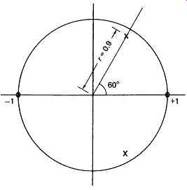
FIG. 66 (a) The peak frequency chosen here is one-sixth of the sample rate,
which requires the poles to be on radii at ±60 from the real axis. The radius
of 0.9 places the poles close to the unit cycle, resulting in a pronounced
peak.
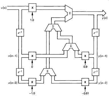
FIG. 66 (b) The biquadratic configuration shown here implements the recurrence
relationship derived in the text: y[n] = x[n]- x[n - 2] + 0.9y[n - 1] - 0.81y[n
- 2].
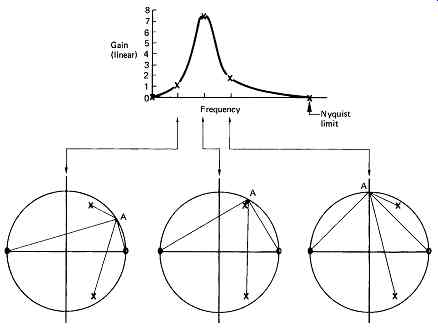
FIG. 66 (c) Calculating the frequency response of the filter of (b). The
method of FIG. 65(c) is used. Note how the pole vector becomes very short as
the resonance is reached. As this is in the denominator, the response is large.
The instability resulting from a pole on or outside the unit circle is thus
clearly demonstrated.
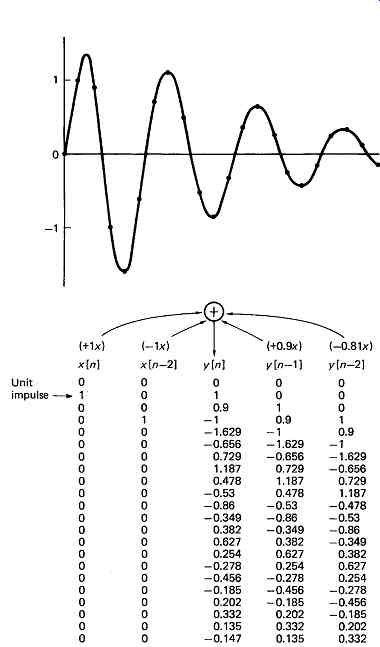
FIG. 66 (d) The response of the filter of (b) to a unit impulse has been
tabulated by using the recurrence relation. The filter rings with a period
of six samples, as expected.
As with the previous example, the frequency response is computed by multiplying the vector lengths, and it will be seen in (c) to have the desired response. The impulse response has been computed for a single non-zero input sample in FIG. 66(d), and this will be seen to ring with a period of six samples as expected.
28. Higher-order filters: cascading
In the example above, the calculations were performed with precision, and the result was as desired. In practice, the coefficients will be represented by a finite wordlength, which means that some inaccuracy will be unavoidable. Owing to the recursion of previous calculations, IIR filters are sensitive to the accuracy of the coefficients, and the higher the order of the filter, the more sensitivity will be shown. In the worst case, a stable filter with a pole near the unit circle may become unstable if the coefficients are represented to less than the required accuracy. Whilst it is possible to design high-order digital filters with a response fixed for a given application, programmable filters of the type required for audio are seldom attempted above the second order to avoid undue coefficient sensitivity. The same response as for a higher-order filter can be obtained by cascading second-order filter sections. For certain applications, such as graphic equalizers, filter sections might be used in parallel.
A further issue which demands attention is the effect of truncation of the wordlength within the data path of the filter. Truncation of coefficients causes only a fixed change in the filter performance which can be calculated. The same cannot be said for data-path truncation. When a sample is multiplied by a coefficient, the necessary wordlength increases dramatically. In a recursive filter the output of one multiplication becomes the input to the next, and so on, making the theoretical wordlength required infinite. By definition, the required wordlength is not available within a realizable filter. Some low-order bits of the product will be lost, which causes noise or distortion depending on the input signal. A series cascade will produce more noise of this kind than a parallel implementation.
In some cases, truncation can cause oscillation. Consider a recursive decay following a large input impulse. Successive output samples become smaller and smaller, but if truncation takes place, the sample may be coarsely quantized as it becomes small, and at some point will not be the correct proportion of the previous sample. In an extreme case, the decay may reverse, and the output samples will grow in magnitude until they are great enough to be represented accurately in the truncation, when they will again decay. The filter is then locked in an endless loop known as a limit cycle.
It is a form of instability which cannot exist on large signals because the larger a signal becomes, the smaller the effect of a given truncation. It can be prevented by the injection of digital dither at an appropriate point in the data path. The randomizing effect of the dither destroys the deterministic effect of truncation and prevents the occurrence of the limit cycle.
In the opposite case from truncation due to losing low-order sample bits, products are also subject to overflow if sufficient high-order bits are not available after a multiplication.
A simple overflow results in a wraparound of the sample value, and is most disturbing as well as being a possible source of large-amplitude limit cycles. The clipping or saturating adders described in section 3 find an application in digital filters, since the output clips or limits instead of wrapping, and limit cycles are prevented. In order to balance the requirements of truncation and saturation, the output of one stage may be shifted one or more binary places before entering the next stage. This process is known as scaling, since shifting down in binary divides by powers of two; it can be used to prevent overflow. Conversely if the coefficients in use dictate that the high-order bits of a given multiplier output will never be exercised, a shift up may be used to reduce the effects of truncation.
The configuration shown in FIG. 66 is not the only way of implementing a two-pole two-zero filter. Fig. 67 shows some alternatives. Starting with the direct form 2 filter, the delays are exchanged with the adders to give a structure which is sometimes referred to as the canonic form.
Filters can also be transposed to yield a different structure with the same transfer function. Transposing is done by reversing signal flow in all the branches, the delays and the multipliers, and replacing nodes in the flow with adders and vice versa. Coefficients and delay lengths are unchanged. The transposed configurations are shown in FIG. 67(b) and (c). The transposed direct form 2 filter has advantages for audio use, 21 since it has less tendency to problems with overflow, and can be made so that the dominant truncation takes place at one node, which eases the avoidance of limit cycles.
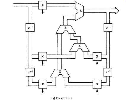
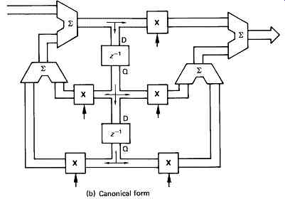
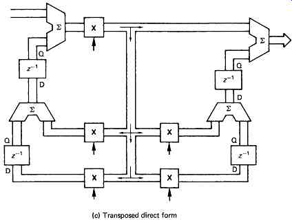
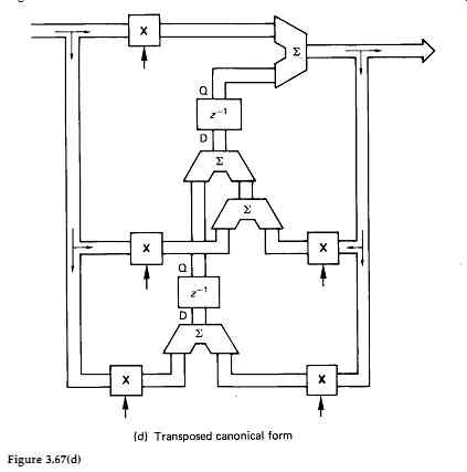
FIG. 67 The same filter can be realized in the direct and canonical forms,
(a) and (b), and each can be transposed, (c) and (d).
29. Pole/zero positions
Since the coefficients of a digital filter are all binary numbers of finite wordlength, it follows that there must be a finite number of positions of poles and zeros in the z-plane. For audio use, the frequencies at which the greatest control is required are usually small compared to the sampling frequency. In presence filters, the requirement for a sharp peak places the poles near to the unit circle, and the low frequencies used emphasize the area adjacent to unity on the real axis. For maximum flexibility of response, a large number of pole and zero positions are needed in this area for given coefficient wordlengths. The structure of the filter has a great bearing on the pole and zero positions available.
Canonic structures result in highly non-uniform distributions of available pole positions, and the direct form is little better.
FIG. 68 shows a comparison of direct form and coupled form, where the latter has a uniform pole distribution. The transfer function of the arrangement of FIG. 68(a) is given by:
H[z]= 1 1+ az-1 + bz-2
Reference to section 27 will show that a = -2rcos_T and b = r2
When poles are near to unit radius, r is nearly 1, and so also is coefficient b. When T is small, a will be nearly -2. In this case a more accurate representation of the coefficients can be had by expressing them as the difference between the wanted values and 1 and -2 respectively.
Thus b becomes 1-b and a becomes 2- a . Since a and b are small, representing them with a reasonable wordlength means that the low order bit represents a much smaller quantizing step with respect to unity.
This is the approach of the Agarwal-Burrus filter structure.
FIG. 69 shows the equivalent of FIG. 68(a) where the use of difference coefficients can be seen. The multiplication by -1 requires only complementing, and by -2 requires a single-bit shift in addition.
An alternative method of providing accurate coefficients is to trans form the z-plane with a horizontal shift, as in FIG. 70(a). A new z plane is defined, where the origin is at unity on the real z-axis:
z
= z -1 and z
-1
=
1 z -1
=
z-1 1- z-1
FIG. 70(b) shows that the above expression is used in the realization of a z stage, which will be seen to be a digital integrator. The general expression for a biquadratic section is given in (c). z - 1 is replaced by 1/(z+ 1) throughout, and the expression is multiplied out. It will be seen that the z-plane coefficients gathered in brackets can be replaced by z -plane coefficients. When poles and zeros are required near Re[z] = 1, it will be found that all the z coefficients are small, allowing accurate multiplication with short-coefficient wordlengths. FIG. 70(d) shows a filter constructed in this way. These configurations demonstrate their accuracy with minimal truncation noise and limit cycles.
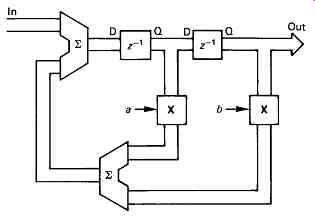
FIG. 68 (a) A second-order, direct-form digital filter, with coefficients
quantized to three bits (not including the sign bit). This means that each
coefficient can have only eight values. As the pole radius is the square root
of the coefficient b the pole distribution is non-uniform, and poles are not
available in the area near to Re[z] = 1 which is of interest in audio.
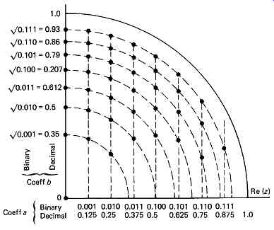
FIG. 68 (b) In the coupled structure shown here, the realizable pole positions
are now on a uniform grid, with the advantage of more pole positions near to
Re[z] = 1, but with the penalty that more processing is required.
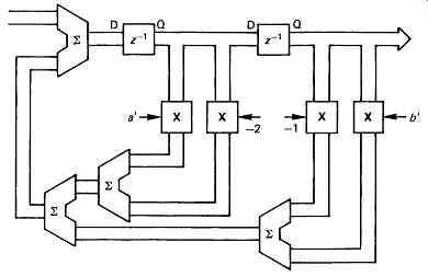
FIG. 69 In the Agarwal-Burrus filter structure, advantage is taken of the
fact that the coefficients are nearly 1 and 2 when the poles are close to unit
radius. The coefficients actually used are the difference between these round
numbers and the desired value. This configuration should be compared with that
of FIG. 68(a).
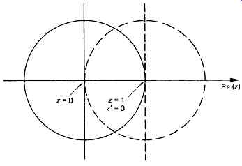
FIG. 70 (a) By defining a new z -plane whose origin is at Re[z] = 1, small
coefficients in z will correspond to poles near to z = 1.
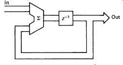
FIG. 70 (b) The above configuration implements a z -1 transfer function.
It is in fact a digital integrator.
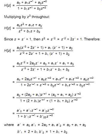
FIG. 70 (c) Conversion to the z -plane requires the coefficients in z to
be combined as shown here.
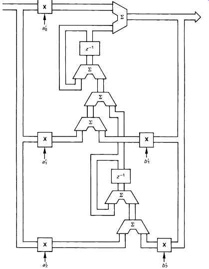
FIG. 70 (d) Implementation of a z-plane filter. The z -1 sections can be
seen at centre. As the coefficients are all small, scaling (not shown) must
be used.
30. The Fourier transform
FIG. 39 showed that if the amplitude and phase of each frequency component is known, linearly adding the resultant components in an inverse transform results in the original waveform. In digital systems the waveform is expressed as a number of discrete samples. As a result the Fourier transform analyses the signal into an equal number of discrete frequencies. This is known as a discrete Fourier transform or DFT in which the number of frequency coefficients is equal to the number of input samples. The fast Fourier transform is no more than an efficient way of computing the DFT.
As was seen in the previous section, practical systems must use windowing to create short-term transforms.
It will be evident from FIG. 71 that the knowledge of the phase of the frequency component is vital, as changing the phase of any component will seriously alter the reconstructed waveform. Thus the DFT must accurately analyze the phase of the signal components.
There are a number of ways of expressing phase. FIG. 72 shows a point which is rotating about a fixed axis at constant speed. Looked at from the side, the point oscillates up and down at constant frequency. The waveform of that motion is a sine wave, and that is what we would see if the rotating point were to translate along its axis whilst we continued to look from the side.
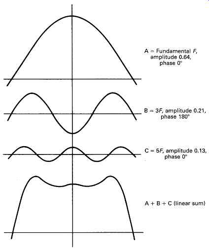
FIG. 71 Fourier analysis allows the synthesis of any waveform by the addition
of discrete frequencies of appropriate amplitude and phase.
One way of defining the phase of a waveform is to specify the angle through which the point has rotated at time zero (T = 0). If a second point is made to revolve at 90 degrees to the first, it would produce a cosine wave when translated. It is possible to produce a waveform having arbitrary phase by adding together the sine and cosine wave in various proportions and polarities. For example, adding the sine and cosine waves in equal proportion results in a waveform lagging the sine wave by 45 degrees.
FIG. 72 shows that the proportions necessary are respectively the sine and the cosine of the phase angle. Thus the two methods of describing phase can be readily interchanged.
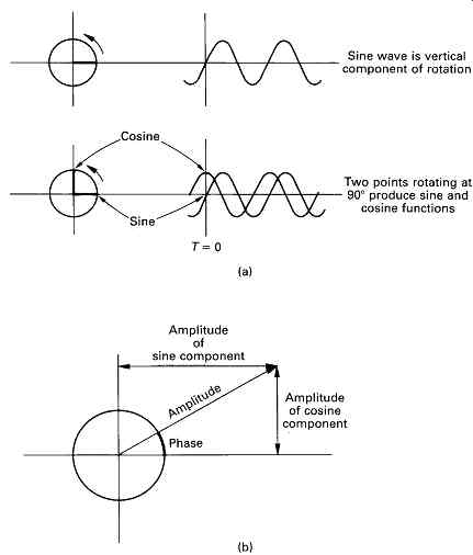
FIG. 72 The origin of sine and cosine waves is to take a particular viewpoint
of a rotation. Any phase can be synthesized by adding proportions of sine and
cosine waves.
The discrete Fourier transform spectrum-analyses a string of samples by searching separately for each discrete target frequency. It does this by multiplying the input waveform by a sine wave, known as the basis function, having the target frequency and adding up or integrating the products. FIG. 73(a) shows that multiplying by basis functions gives a non-zero integral when the input frequency is the same, whereas (b) shows that with a different input frequency (in fact all other different frequencies) the integral is zero showing that no component of the target frequency exists. Thus from a real waveform containing many frequencies all frequencies except the target frequency are excluded. The magnitude of the integral is proportional to the amplitude of the target component.
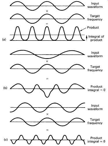
FIG. 73 The input waveform is multiplied by the target frequency and the
result is averaged or integrated. At (a) the target frequency is present and
a large integral results.
With another input frequency the integral is zero as at (b). The correct frequency will also result in a zero integral shown at (c) if it is at 90° to the phase of the search frequency. This is overcome by making two searches in quadrature.
FIG. 73(c) shows that the target frequency will not be detected if it is phase shifted 90 degrees as the product of quadrature waveforms is always zero. Thus the discrete Fourier transform must make a further search for the target frequency using a cosine basis function. It follows from the arguments above that the relative proportions of the sine and cosine integrals reveals the phase of the input component. Thus each discrete frequency in the spectrum must be the result of a pair of quadrature searches.
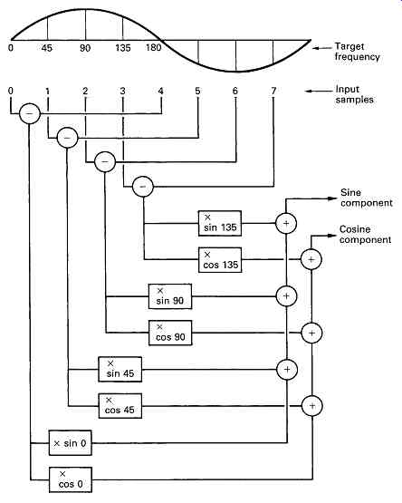
FIG. 74 An example of a filtering search. Pairs of samples are subtracted
and multiplied by sampled sine and cosine waves. The products are added to
give the sine and cosine components of the search frequency.
Searching for one frequency at a time as above will result in a DFT, but only after considerable computation. However, a lot of the calculations are repeated many times over in different searches. The fast Fourier transform gives the same result with less computation by logically gathering together all the places where the same calculation is needed and making the calculation once.
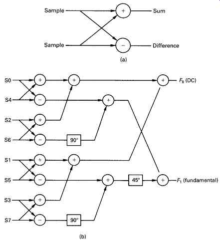
FIG. 75 The basic element of an FFT is known as a butterfly as at (a) because
of the shape of the signal paths in a sum and difference system. The use of
butterflies to compute the first two coefficients is shown in (b).
The amount of computation can be reduced by performing the sine and cosine component searches together. Another saving is obtained by noting that every 180 degrees the sine and cosine have the same magnitude but are simply inverted in sign. Instead of performing four multiplications on two samples 180 degrees apart and adding the pairs of products it is more economical to subtract the sample values and multiply twice, once by a sine value and once by a cosine value.
The first coefficient is the arithmetic mean which is the sum of all the sample values in the block divided by the number of samples. FIG. 74 shows how the search for the lowest frequency in a block is performed.
Pairs of samples are subtracted as shown, and each difference is then multiplied by the sine and the cosine of the search frequency. The process shifts one sample period, and a new sample pair are subtracted and multiplied by new sine and cosine factors. This is repeated until all the sample pairs have been multiplied. The sine and cosine products are then added to give the value of the sine and cosine coefficients respectively.
It is possible to combine the calculation of the DC component which requires the sum of samples and the calculation of the fundamental which requires sample differences by combining stages shown in FIG. 75(a) which take a pair of samples and add and subtract them. Such a stage is called a butterfly because of the shape of the schematic. FIG. 75(b) shows how the first two components are calculated. The phase rotation boxes attribute the input to the sine or cosine component outputs according to the phase angle. As shown the box labeled 90 degrees attributes nothing to the sine output, but unity gain to the cosine output.
The 45 degree box attributes the input equally to both components.
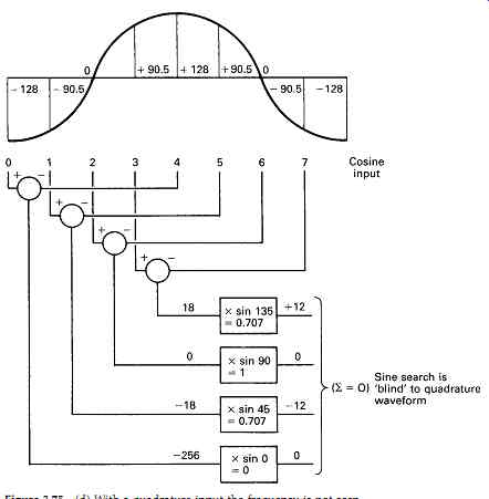
FIG. 75 (c) An actual calculation of a sine coefficient. This should be compared
with the result shown in (d).
FIG. 75 (d) With a quadrature input the frequency is not seen.
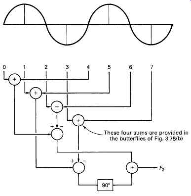
FIG. 75 (e) The butterflies used for the first coefficients form the basis
of the computation of the next coefficient.
FIG. 75(c) shows a numerical example. If a sinewave input is considered where zero degrees coincides with the first sample, this will produce a zero sine coefficient and non-zero cosine coefficient. FIG. 75(d) shows the same input waveform shifted by 90 degrees. Note how the coefficients change over.
FIG. 75(e) shows how the next frequency coefficient is computed.
Note that exactly the same first-stage butterfly outputs are used, reducing the computation needed.
A similar process may be followed to obtain the sine and cosine coefficients of the remaining frequencies. The full FFT diagram for eight samples is shown in FIG. 76(a). The spectrum this calculates is shown in (b). Note that only half of the coefficients are useful in a real band limited system because the remaining coefficients represent frequencies above one half of the sampling rate.
In short-time Fourier transforms (STFTs) the overlapping input sample blocks must be multiplied by window functions. The principle is the same as for the application in FIR filters shown in section 23. FIG. 77 shows that multiplying the search frequency by the window has exactly the same result except that this need be done only once and much computation is saved. Thus in the STFT the basis function is a windowed sine or cosine wave.
The FFT is used extensively in such applications as phase correlation, where the accuracy with which the phase of signal components can be analyzed is essential. It also forms the foundation of the discrete cosine transform.
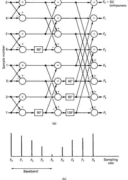
FIG. 76 At (a) is the full butterfly diagram for an FFT. The spectrum this
computes is shown at (b).
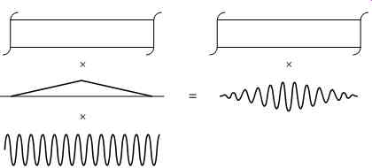
FIG. 77 Multiplication of a windowed block by a sine wave basis function
is the same as multiplying the raw data by a windowed basis function but requires
less multiplication as the basis function is constant and can be pre-computed.
31. The discrete cosine transform (DCT)
The DCT is a special case of a discrete Fourier transform in which the sine components of the coefficients have been eliminated leaving a single number. This is actually quite easy. FIG. 78(a) shows a block of input samples to a transform process. By repeating the samples in a time-reversed order and performing a discrete Fourier transform on the double-length sample set a DCT is obtained. The effect of mirroring the input waveform is to turn it into an even function whose sine coefficients are all zero. The result can be understood by considering the effect of individually transforming the input block and the reversed block.
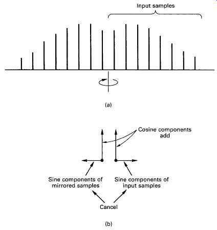
FIG. 78 The DCT is obtained by mirroring the input block as shown at (a) prior
to an FFT. The mirroring cancels out the sine components as at (b), leaving
only cosine coefficients.
FIG. 78(b) shows that the phase of all the components of one block are in the opposite sense to those in the other. This means that when the components are added to give the transform of the double length block all the sine components cancel out, leaving only the cosine coefficients, hence the name of the transform.
In practice the sine component calculation is eliminated. Another advantage is that doubling the block length by mirroring doubles the frequency resolution, so that twice as many useful coefficients are produced. In fact a DCT produces as many useful coefficients as input samples.
32. The wavelet transform
The wavelet transform was not discovered by any one individual, but has evolved via a number of similar ideas and was only given a strong mathematical foundation relatively recently.
The wavelet transform is similar to the Fourier transform in that it has basis functions of various frequencies which are multiplied by the input waveform to identify the frequencies it contains. However, the Fourier transform is based on periodic signals and endless basis functions and requires windowing. The wavelet transform is fundamentally windowed, as the basis functions employed are not endless sine waves, but are finite on the time axis; hence the name. Wavelet transforms do not use a fixed window, but instead the window period is inversely proportional to the frequency being analyzed. As a result a useful combination of time and frequency resolutions is obtained. High frequencies corresponding to transients in audio or edges in video are transformed with short basis functions and therefore are accurately located. Low frequencies are transformed with long basis functions which have good frequency resolution.
FIG. 79 shows that that a set of wavelets or basis functions can be obtained simply by scaling (stretching or shrinking) a single wavelet on the time axis. Each wavelet contains the same number of cycles such that as the frequency reduces, the wavelet gets longer. Thus the frequency discrimination of the wavelet transform is a constant fraction of the signal frequency. In a filter bank such a characteristic would be described as 'constant Q'. FIG. 80 shows the division of the frequency domain by a wavelet transform is logarithmic whereas in the Fourier transform the division is uniform. The logarithmic coverage is effectively dividing the frequency domain into octaves and as such parallels the frequency discrimination of human hearing.
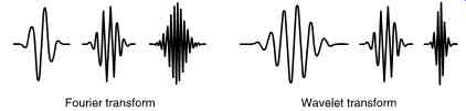
FIG. 79 Unlike discrete Fourier transforms, wavelet basis functions are scaled
so that they contain the same number of cycles irrespective of frequency. As
a result their frequency discrimination ability is a constant proportion of
the centre frequency.
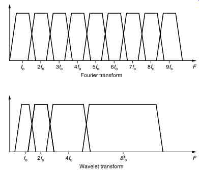
FIG. 80 Wavelet transforms divide the frequency domain into octaves instead
of the equal bands of the Fourier transform.
As it is relatively recent, the wavelet transform has yet to be widely used although it shows great promise. It has been successfully used in audio and in commercially available non-linear video editors and in other fields such as radiology and geology.
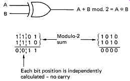
FIG. 81 In modulo-2 calculations, there can be no carry or borrow operations
and conventional addition and subtraction become identical. The XOR gate is
a modulo-2 adder.
33. Modulo-n arithmetic
Conventional arithmetic which is in everyday use relates to the real world of counting actual objects, and to obtain correct answers the concepts of borrow and carry are necessary in the calculations.
There is an alternative type of arithmetic which has no borrow or carry which is known as modulo arithmetic. In modulo-n no number can exceed n. If it does, n or whole multiples of n are subtracted until it does not. Thus 25 modulo-16 is 9 and 12 modulo-5 is 2. The count shown in FIG. 81 is from a four-bit device which overflows when it reaches 1111 because the carry-out is ignored. If a number of clock pulses m are applied from the zero state, the state of the counter will be given by m mod.16. Thus modulo arithmetic is appropriate to systems in which there is a fixed wordlength and this means that the range of values the system can have is restricted by that wordlength. A number range which is restricted in this way is called a finite field.
Modulo-2 is a numbering scheme which is used frequently in digital processes. FIG. 81 also shows that in modulo-2 the conventional addition and subtraction are replaced by the XOR function such that: A + B Mod.2 = A XOR B. When multi-bit values are added Mod.2, each column is computed quite independently of any other. This makes Mod.2 circuitry very fast in operation as it is not necessary to wait for the carries from lower-order bits to ripple up to the high-order bits.
Modulo-2 arithmetic is not the same as conventional arithmetic and takes some getting used to. For example, adding something to itself in Mod.2 always gives the answer zero.
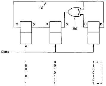
FIG. 82 The circuit shown is a twisted-ring counter which has an unusual
feedback arrangement. Clocking the counter causes it to pass through a series
of non-sequential values. See text for details.
34. The Galois field
FIG. 82 shows a simple circuit consisting of three D-type latches which are clocked simultaneously. They are connected in series to form a shift register. At (a) a feedback connection has been taken from the output to the input and the result is a ring counter where the bits contained will recirculate endlessly. At (b) one XOR gate is added so that the output is fed back to more than one stage. The result is known as a twisted-ring counter and it has some interesting properties. Whenever the circuit is clocked, the left-hand bit moves to the right-hand latch, the centre bit moves to the left-hand latch and the centre latch becomes the XOR of the two outer latches. The figure shows that whatever the starting condition of the three bits in the latches, the same state will always be reached again after seven clocks, except if zero is used.
The states of the latches form an endless ring of non-sequential numbers called a Galois field after the French mathematical prodigy Evariste Galois who discovered them. The states of the circuit form a maximum-length sequence because there are as many states as are permitted by the wordlength. As the states of the sequence have many of the characteristics of random numbers, yet are repeatable, the result can also be called a pseudo-random sequence (prs). As the all-zeros case is disallowed, the length of a maximum length sequence generated by a register of m bits cannot exceed (2m-1) states. The Galois field, however includes the zero term. It is useful to explore the bizarre mathematics of Galois fields which use modulo-2 arithmetic. Familiarity with such manipulations is helpful when studying the error correction, particularly the Reed-Solomon codes used in recorders and treated in section 6.
They will also be found in processes which require pseudo-random numbers such as digital dither, treated in section 14, and randomized channel codes used in, for example, NICAM 728 and discussed in sections 6 and 8.
The circuit of FIG. 82 can be considered as a counter and the four points shown will then be representing different powers of 2 from the MSB on the left to the LSB on the right. The feedback connection from the MSB to the other stages means that whenever the MSB becomes 1, two other powers are also forced to one so that the code of 1011 is generated.
Each state of the circuit can be described by combinations of powers of x, such as x2
= 100, x = 010, x2
+ x = 110, etc.
The fact that three bits have the same state because they are connected together is represented by the Mod.2 equation:
x3 + x + 1=0 Let x = a, which is a primitive element. Now a3 + a + 1 = 0
(1) In modulo
2 a + a = a2 + a2 =0
a = x = 010 a2
= x2
= 100 a3
= a + 1 = 011 from (1) a4
= a _ a3
= a(a + 1) = a2 + a =110 a5
= a2
+ a + 1 = 111 a6
= a _ a5
= a(a2 + a + 1)
= a3 + a2 + a = a + 1 + a2 + a
= a2 + 1 = 101 a7
= a(a2 + 1) = a3 + a
= a + 1 + a =1=001
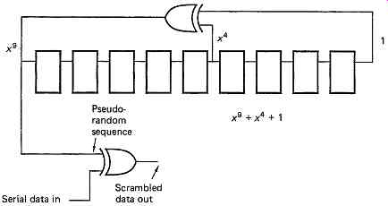
FIG. 83 In NICAM, randomizing is done by adding the serial data to a polynomial
generated by the circuit shown here. The receiver needs an identical system
which is synchronous with that of the transmitter.
In this way it can be seen that the complete set of elements of the Galois field can be expressed by successive powers of the primitive element. Note that the twisted-ring circuit of FIG. 82 simply raises a to higher and higher powers as it is clocked; thus the seemingly complex multibit changes caused by a single clock of the register become simple to calculate using the correct primitive and the appropriate power.
The numbers produced by the twisted-ring counter are not random; they are completely predictable if the equation is known. However, the sequences produced are sufficiently similar to random numbers that in many cases they will be useful. They are thus referred to as pseudo random sequences. The feedback connection is chosen such that the expression it implements will not factorize. Otherwise a maximum length sequence could not be generated because the circuit might sequence around one or other of the factors depending on the initial condition. A useful analogy is to compare the operation of a pair of meshed gears. If the gears have a number of teeth which is relatively prime, many revolutions are necessary to make the same pair of teeth touch again. If the number of teeth have a common multiple, far fewer turns are needed.
FIG. 83 shows the pseudo-random sequence generator used in NICAM 728. Its purpose is to break up the transmitted spectrum so that the sound carrier does not cause patterning on the TV picture. The sequence length of the circuit shown is 511 because the expression will not factorize. Further details of NICAM 728 can be found in section 8.
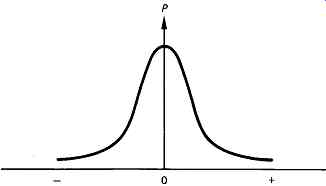
FIG. 84 White noise in analog circuits generally has the Gaussian amplitude
distribution.
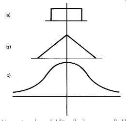
FIG. 85 At (a) is a rectangular probability; all values are equally likely
but between physical limits. At (b) is the sum of two rectangular probabilities,
which is triangular, and at (c) is the Gaussian curve which is the sum of an
infinite number of rectangular probabilities.
35. Noise and probability
Probability is a useful concept when dealing with processes which are not completely predictable. Thermal noise in electronic components is random, and although under given conditions the noise power in a system may be constant, this value only determines the heat that would be developed in a resistive load. In digital systems, it is the instantaneous voltage of noise which is of interest, since it is a form of interference which could alter the state of a binary signal if it were large enough.
Unfortunately the instantaneous voltage cannot be predicted; indeed if it could the interference could not be called noise. Noise can only be quantified statistically, by measuring or predicting the likelihood of a given noise amplitude.
FIG. 84 shows a graph relating the probability of occurrence to the amplitude of noise. The noise amplitude increases away from the origin along the horizontal axis, and for any amplitude of interest, the probability of that noise amplitude occurring can be read from the curve.
The shape of the curve is known as a Gaussian distribution, which crops up whenever the overall effect of a large number of independent phenomena is considered. Thermal noise is due to the contributions from countless molecules in the component concerned. Magnetic recording depends on superimposing some average magnetism on vast numbers of magnetic particles.
If it were possible to isolate an individual noise-generating microcosm of a tape or a head on the molecular scale, the noise it could generate would have physical limits because of the finite energy present. The noise distribution might then be rectangular as shown in FIG. 85(a), where all amplitudes below the physical limit are equally likely. The output of a twisted-ring counter such as that in FIG. 82 can have a uniform probability. Each value occurs once per sequence. The outputs are positive only but do not include zero, but every value from 1 up to 2n-1 is then equally likely.
The output of a prs generator can be made into the two's complement form by inverting the MSB. This has the effect of exchanging the missing all zeros value for a missing fully negative value as can be seen by considering the number ring in FIG. 5. In this example, inverting the MSB causes the code of 1000 representing -8 to become 0000. The result is a four-bit prs generating uniform probability from -7 to +7 as shown in FIG. 85(a).
If the combined effect of two of these uniform probability processes is considered, clearly the maximum amplitude is now doubled, because the two effects can add, but provided the two effects are uncorrelated, they can also subtract, so the probability is no longer rectangular, but becomes triangular as in FIG. 85(b). The probability falls to zero at peak amplitude because the chances of two independent mechanisms reaching their peak value with the same polarity at the same time are understandably small.
If the number of mechanisms summed together is now allowed to increase without limit, the result is the Gaussian curve shown in FIG. 85(c), where it will be seen that the curve has no amplitude limit, because it is just possible that all mechanisms will simultaneously reach their peak value together, although the chances of this happening are incredibly remote. Thus the Gaussian curve is the overall probability of a large number of uncorrelated uniform processes.
References
1. Spreadbury, D., Harris, N. and Lidbetter, P. So you think performance is cracked using standard floating point DSPs? Proc. 10th. Int. AES Conf., 105-110 (1991)
2. Richards, J.W., Digital audio mixing. The Radio and Electron. Eng., 53, 257-264 (1983)
3. Richards, J.W. and Craven, I., An experimental 'all digital' studio mixing desk. J. Audio Eng. Soc., 30, 117-126 (1982)
4. Jones, M.H., Processing systems for the digital audio studio. In Digital Audio, edited by B. Blesser, B. Locanthi and T.G. Stockham Jr, pp. 221-225, New York: Audio Engineering Society (1982)
5. Lidbetter, P.S., A digital delay processor and its applications. Presented at the 82nd Audio Engineering Society Convention (London, 1987), Preprint 2474(K-4)
6. McNally, G.J., COPAS A high speed real time digital audio processor. BBC Research Dept Report, RD 1979/26
7. McNally, G.W., Digital audio: COPAS-2, a modular digital audio signal processor for use in a mixing desk. BBC Research Dept Report, RD 1982/13
8. Vandenbulcke, C. et al., An integrated digital audio signal processor. Presented at the 77th Audio Engineering Society Convention (Hamburg, 1985), Preprint 2181(B-7)
9. Moorer, J.A., The audio signal processor: the next step in digital audio. In Digital Audio, edited by B. Blesser, B. Locanthi and T.G. Stockham Jr, pp. 205-215, New York: Audio Engineering Society (1982)
10. Gourlaoen, R. and Delacroix, P., The digital sound mixing desk: architecture and integration in the future all-digital studio. Presented at the 80th Audio Engineering Society Convention (Montreux, 1986), Preprint 2327(D-1)
11. Ray, S.F., Applied Photographic Optics. Oxford: Focal Press (1988) (Ch. 17)
12. van den Enden, A.W.M. and Verhoeckx, N.A.M., Digital signal processing: theoretical background. Philips Tech. Rev., 42, 110-144, (1985)
13. McClellan, J.H., Parks, T.W. and Rabiner, L.R., A computer program for designing optimum FIR linear-phase digital filters. IEEE Trans. Audio and Electroacoustics, AU-21, 506-526 (1973)
14. Dolph, C.L., A current distribution for broadside arrays which optimizes the relationship between beam width and side lobe level. Proc. IRE, 34, 335-348 (1946)
15. Crochiere, R.E. and Rabiner, L.R., Interpolation and decimation of digital signals - a tutorial review. Proc. IEEE, 69, 300-331 (1981)
16. Rabiner, L.R., Digital techniques for changing the sampling rate of a signal. In Digital Audio, edited by B. Blesser, B. Locanthi and T.G. Stockham Jr, pp. 79-89, New York: Audio Engineering Society (1982)
17. Lagadec, R., Digital sampling frequency conversion. In Digital Audio, edited by B. Blesser, B. Locanthi and T.G. Stockham Jr, pp. 90-96, New York: Audio Engineering Society (1982)
18. Jackson, L.B., Roundoff noise analysis for fixed-point digital filters realized in cascade or parallel form. IEEE Trans. Audio and Electroacoustics, AU-18, 107-122 (1970)
19. Parker, S.R., Limit cycles and correlated noise in digital filters. In Digital Signal Processing, Western Periodicals Co., 177-179 (1979)
20. Claasen, T.A.C.M., Mecklenbrauker, W.F.G. and Peek, J.B.H., Effects of quantizing and overflow in recursive digital filters. IEEE Trans. ASSP, 24, 517-529 (1976)
21. McNally, G.J., Digital audio: recursive digital filtering for high-quality audio signals. BBC Res. Dept Report, RD 1981/10
22. Rabiner, L.R. and Gold, B., Theory and Application of Digital Signal Processing, New Jersey: Prentice Hall (1975)
23. Agarwal, R.C. and Burrus, C.S., New recursive digital filter structures having very low sensitivity and roundoff noise. IEEE Trans. Circuits. Syst., CAS-22, 921-927 (1975)
24. Kraniauskas, P., Transforms in Signals and Systems, Wokingham: Addison-Wesley (1992)
25. Ahmed, N., Natarajan, T. and Rao, K., Discrete Cosine Transform, IEEE Trans. Computers, C-23 90-93 (1974)
26. Goupillaud, P., Grossman, A. and Morlet, J., Cycle-Octave and related transforms in seismic signal analysis. Geoexploration, 23, 85-102, Elsevier Science (1984/5)
27. Daubechies, I., The wavelet transform, time-frequency localisation and signal analysis. IEEE Trans. Info. Theory, 36, No.5, 961-1005 (1990)
28. Rioul, O. and Vetterli, M., Wavelets and signal processing. IEEE Signal Process. Mag., 14-38 (Oct. 1991) 29. Strang, G. and Nguyen, T., Wavelets and Filter Banks, Wellesly, MA: Wellesley-Cambridge Press (1996)
++++++++