Digital Techniques in Sound Reproduction-- Part II (May 1980)

by Daniel Minoli [International Telephone and Telegraph Domestic Transmission Systems, Inc. New York, N.Y.]

Signal Processing

The advances in acoustic signal processing techniques we describe below have been brought about by the needs of the telecommunications industry to provide (relatively) noise-free telephony over ultra-long distance (intercontinental) calls and to achieve better throughput from existing facilities.

Before we proceed further into signal processing aspects, which is the key subject of this article, we want to point out that computers (which, as discussed in Part I, speak only digital language) also must communicate to distant locations via telephone lines. To do this, and here is the amusing point, computers still in large part must convert this digital stream into an analog stream--the telephone does not transmit square waves very far. A device to do this coding at one end and decoding at the other is called modem and operates (in its simplest form) by coding a 0 with a single sine wave tone at 2025 hertz and a 1 with a sine wave of 2225 hertz. In the telephone audio band, this is all that is required to achieve communication.

How, then, can a wave be converted to and from digital form so the advantages of digital processing can be realized? Broadly speaking, there are two approaches to the conversion problem. Waveform digitization methods take samples of the waveform and represent the sampled waveform amplitudes by digital, binary-coded values. At the other end, the digital signals are converted back to analog form in an attempt to reconstruct the original speech waveform. As the name implies, these coders essentially strive for facsimile reproduction of the signal waveform. In principle, they are designed to be signal-independent, hence they can code equally well a variety of signals--speech, music, tones, wideband data. In contrast, vocoder methods make no at tempt to preserve the original speech waveform. Instead, the input signal is analyzed in terms of standardized features, each of which can be transmitted in digitally coded form. At the other end, these features are reassembled and an output signal is synthesized [3.] The vocoder approach is finding excellent applications to the transmission of speech, particularly where extremely low bandwidth (20 Hz to 1000 Hz or approximately 50 to 2400 bits per second) is needed and for secure, encrypted applications.

These devices are still very expensive ($12,000-$15,000 and up), and the underlying techniques cannot be used in a general musical context unless (1) one either knows exactly the instrument playing and this must be in a solo application since the vocoder is tailored after the acoustic entity it is trying to synthesize, or (2) one uses a vocoder to get a synthetic voice--say synthetic operatic voices (do not confuse this with any of the existing musical synthesizers; to my knowledge, no one has yet tried what we advocate here).

Before we continue, let's look at a graphic example which makes the distinction between the two methods unequivocal. Think of waveform coding techniques, such as pulse code modulation (PCM), as cooking a delectable cake in Par is, then using an SST to carry the cake to New York, in a well-heated oven, for delivery to a fancy restaurant. Think of vocoder techniques as getting in touch with a renowned cook in Paris, writing down his recipe on a piece of paper, mailing the recipe to the New York restaurant we are considering, and baking the cake in New York. The benefits/drawbacks of each method are clear. The first is clumsy and requires a lot of space and special handling, but you get the original, authentic product. The second method is elegant, concise, and quick, but you get a replica (not always 100 percent faithful) of the product.

Interestingly, a software/hardware trade-off between the two approaches exists. Assume we were thinking of coding human voice, so that the vocoder could be used; suppose also we needed to put 20 hours of speech on some software disc. If we use vocoders, the recording/reproducing hard ware would be expensive, but the software would be cheap since you could put the entire 20 hours on a single disc (by assumption). If we use PCM, the recording/reproducing hardware is inexpensive (we only basically need A/D, D/A devices as described below), but the software would be ex pensive since you now need 20 discs to store the same information. This type of trade-off consideration is done everyday in the telecommunications industry: If the call has to go across town, use PCM; if it has to go to Europe, vocoder techniques may be more cost effective.

A digital audio system can be viewed as containing six distinct sections--input analog, analog-to-digital conversion, digital processing, digital storage, digital-to-analog con version, and output analog. By comparison an analog/digital/analog system is composed as follows, input analog, A/D conversion, digital processing, D/A conversion, analog storage, analog output. Although the two conversion subsections can be designed using any number of waveform coding techniques, they can all be analyzed as information transformations between the analog and digital domains. This provides a unifying structure for examining conversion without regard to implementation.

The analog world (or domain) is characterized by variables that can take any value within a specified range; for example the temperature can be 65, 65.21, 65.211723 degrees F., etc.; an electrical current can be 0.5, 0.55, 0.5592662, 0.5592663 V.

(However, if we add the concept of analog noise, then the resolution cannot be any better than the noise value. If, for example, the noise magnitude was on the order of 0.001 V, we might elect to say that the last two voltages could be considered as having originated from the same "true" value and that the difference can be attributed to noise; the additive noise limits the analog resolution in that the ability to distinguish two voltages is impaired by noise.) We can say that infinitely many values can be assured by the analog vari able.

We have already seen that in the digital domain we can only represent a finite set of values: The size of this set, and the preciseness (significance) of the digital quantity is a function of the code we have elected to use. With two bits we can represent four numbers; these can be:

00=0, 01=1, 10= 2, 11=3; or 00=0,0.1 = 0.5, 1.0 = 1, 1.1 = 1.5; or .00 = 0, .01 = 0.25, .10 = 0.50, and .11 = 0.75.

If we need more resolution or range, we need more bits.

In order for each digital word to represent a signal that originated in the analog domain, each word is assigned to a region of the analog signal range. This requires that the analog domain be divided (quantized) into the same number of regions as there are digital words. Consider an analog signal ranging between 0 and +1 V which is to be mapped on to a 4-bit word. This requires that the one-volt range be divided into 16 regions, as illustrated in Fig. 11. Since we made each of the quantization regions the same size, in this example the levels are spaced at intervals of 0.0625 V. Any voltage be tween 0.975 and 1.0000 V would be assigned a unique word such as 1111. (The spacing need not be uniform; this is referred to as "companding" or compression/expansion, which is logarithmic PCM). Since all other voltages in this interval are represented by the same word, we can say that the quantization process creates an error, called quantization error. Clearly, adding another bit to the digital word would allow twice as many levels to be specified, and the quantization error would be cut in half.

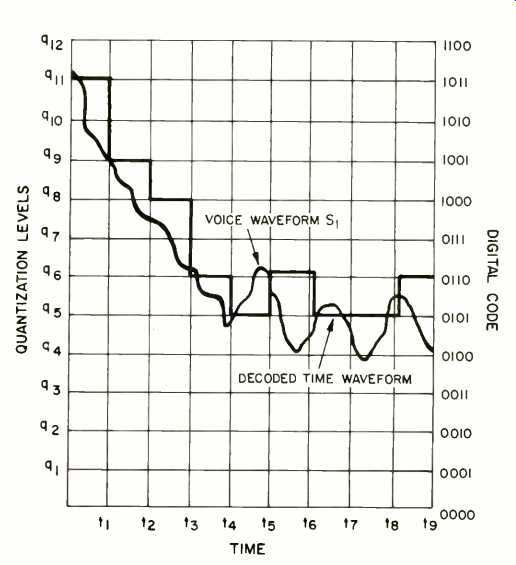
Fig. 11--Pulse code modulation (PCM).

Increasing the number of bits can reduce this error significantly, but there must always be an error since there are a discrete number of exact analog voltages represented by the digital words but an infinite number of analog voltages [4].

Another way of seeing this form of encoding is as follows:

We move along the curve and at every point or, at least, a large number of points, we measure and write down the height of the curve from the X axis, but we must remember four things: (1) Our yardstick does not allow us to measure, say, 7.32172, but only 7.321 (quantization error); (2) The marks on our yardstick are a function of the number of codes we have available (word length); (3) We can't measure every point and must settle for a subset (sampling), and (4) Since our numbers must be used by a computer, they must be written in digital (101101 V) rather than decimal (45 V) form.

Discrete Time Sampling

The previous discussion considered the mapping of a single analog voltage into a single digital word. However, the audio signal is time varying, requiring us to partition the continuous time variable into a discrete series of time points. At each of the time points; referred to as sampling times, the analog voltage is converted into a digital word. Thus, a sequence of digital words is generated at the same rate as the sampling [4].

The concepts of discrete time and quantized amplitude are not the same. Quantization describes the process of collapsing a group of voltages into a single value, whereas discrete sampling means that only specific values of the time variable are being considered. All changes in the analog signal be tween discrete sampling times are ignored. Fortunately, if the analog signal is band limited relative to the sampling rate (Nyquist rate), the information in the sampled analog values is identical to that contained in the complete unsampled analog signal. Even though the sampling process ignores all signal changes between samples, no information is lost. There fore, sampling done the right way preserves all information, while quantization always discards information [4].

How, then, does one sample the signal the right way to retain all the information and thereby reconstruct the original quantized signal? It can be shown mathematically that if the signal has a spectrum which is band limited to one maxi mum top frequency, that is to say, there is absolutely no energy above this frequency (and by definition none below the lower limit), then the number of samples per second must be equal to 2f_max. This is called the Nyquist rate. Restating this, we can say that with a typical 50-kHz sampling frequency, there must be no energy in the original wave above 25 kHz.

The only way that the analog signal can be band limited is by the use of a very sharp low-pass filter before the sampling process. It is therefore the low-pass filtering which destroys information (bandwidth reduction) rather than the sampling process. This is preferable since the low-pass filter merely removes higher frequency components above the Nyquist frequency, whereas the sampling process would generate new frequencies. The only sources of degradation are the low-pass filtering and the quantization process at the input.

It is not the digitization process which creates the degradation: A band limited time-sampled quantized analog signal has the identical information as the sequence of digital words (see Fig. 12) [4].

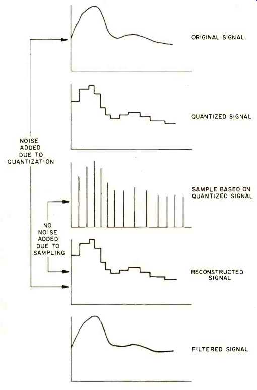
Fig. 12--Conversion steps.

Complete Conversion System

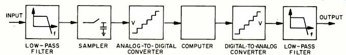
Fig. 13--End-to-end digital system.

A complete digitized audio system is shown in Fig. 13. The incoming analog signal is low-passed with a very sharp filter to restrict the bandwidth as discussed above. This signal is then sampled, and each sample is held to allow the analog-to-digital (A/D) converter time to convert the information into a digital word. Once in the digital domain, the digital processor can perform any number of functions such as de lay, transmission, storage, filtering, compression, or reverberation. At the output, the reverse process takes place: A sequence of digital words is converted to a discrete series of analog voltages by the digital-to-analog (D/A) converter. An output low-pass filter smoothes the discrete analog samples back to a smooth waveform [4].

A/D and D/A converters are inexpensive devices. A D/A converter in a home digital system could cost at most $100; for telephone-grade service, such a device can be purchased for as little as $10.

Signal-to-Quantization Error Ratio

One of the important measures of quality for a digital con version system is the ratio of the maximum signal to the quantization error. This ratio is a function of the number of bits in the conversion. For a signal quantized with an n-bit word system, the signal-to-noise ratio is √ 1.5 x 2^n which becomes the following, in decibels, 6.02n + 1.76. Each bit con tributes six decibels to the system performance.

Some other technical considerations must be given to fully describe the amount of final distortion we would hear in a totally digital system; [4] is the best work yet on this subject.

Out of scientific fairness we have talked at length about the distortion produced by the system; we should, however, emphasize the enormous improvements achievable by digital techniques over conventional or even direct-to-disc techniques.

Let us look at some performance specs for analog-digital-analog discs.

Telarc/Soundstream

1. Frequency Response: D.C. to 21 kHz.
2. THD: Less than 0.004 percent; at peak level, less than 0.03 percent.
3. S/N: 90 dB.
4. Dynamic Range: 90 dB.
5. Sampling Rate: 50,000/S, 16-bit linear PCM.
6. Wow and Flutter: Unmeasurable.

Denon

1. Frequency Response: D.c. to 19 kHz, ±0.2 dB.
2. THD: Less than 0.1 percent.
3. Interchannel Crosstalk: -80 dB.
4. Dynamic Range: 89 dB.
5. Sampling Rate: 47,250/S, 14-bit linear PCM.
6. Wow and Flutter: Unmeasurable.

Philips 4 1/2-in. Digital Disc (Announced)

1. Stereo Program: One hour.
2. Interchannel Crosstalk: -80 dB.
3. S/N: 85 dB.
4. Sampling Rate: Unknown, but greater than 40,000/S, 14-bit PCM.

To quote from Edward Tatnall Canby in his Audio September, 1979, "Audio ETC" column:

----

...The specs for the [Philips] Compact Disc are not quite up to top professional standards--that is, digital standards. Philips is thinking consumer.

Most professional digital tape now uses a 16-bit coding, for the ultimate in "headroom." Philips has made a mild cut back, from 16-bit to 14-bit coding. This allows for a system usable in the very lowest, cheapest popular equipment on a mass basis. But is it a serious compromise from the audio viewpoint? Well, not exactly. Merely from the astronomical to the semi-astronomical. As we are aware, the digital system does not "read" noise of the all-too-familiar analog sort, on either disc or tape.

To be sure, S/N in the Compact Disc system is not quite up to professional digital tape. Instead of an incredible 90 dB down for the noise level, it is reduced to a mere 85 dB.

Please note that the very best an LP can do, in theory, is around 60 dB signal to noise, and we'll say nothing about the average disc. And look at the S/N specs for your hi-fi circuitry, where the noise is purely electronic. This little disc matches the fanciest. Its available dynamic range, to match, is also 85 dB-check that against cassette and LP.

Stereo separation? Because the two stereo channels are read out in separate digital "words" the separation is, well, not quite infinite. The finest stereo cartridges edge up towards a 40-dB channel separation and anything in the mid-30s is very OK for the better models. The Compact Disc figure: 80 dB.

Need I say more about audio quality? It is sensational, and that is that. And yet still, in the end, this disc is potentially inexpensive enough to go into the cheapest of popular mini-players. It has that potential, like its cassette sibling.

----

Those of us lucky enough to own a good system (analog digital-analog discs do indeed tax your system to an unprecedented level, as a note in one of Telarc's records cautions) must say that such recordings sound spectacular. Low-frequency notes come through uncompromised. This response of d.c. to 20 kHz, ±0 dB, is nothing miraculous in digital recordings; it can best be understood if we think of the spectrum of a signal, namely a graph in the amplitude-frequency domain, depicting the power of each frequency component.

In the coding process, low frequencies are as any other frequency; if a 20-Hz note has one watt of power, the coding algorithm so notes that information (effectively); for PCM it is not any different than observing that a 1-kHz note has one watt of power.

It should be remembered that at 50,000 samples per second and 16 bits per sample, one second of music needs 800,000 bits of information (0.8 x10^6 bytes/S); 20 minutes of program require 120 million bytes (1 byte = 8 bits), the size of a typical disk pack attached to a medium-sized minicomputer system. This is a rather large amount of data even by today's standards and why, as we have indicated, we must use the principles of the video disc (another bit-waster), which provides the required bandwidth (it, in fact, can give you about 12 x 10^6 bits/S of storage).

While some end-to-end digital systems already exist or are about to be announced, their introduction will be marked by lack of standardization. For the next two to five years it is safe to assume that A-D-A (analog-digital-analog) processed discs will be the avenue via which most audiophiles will come in contact with digital material (let us hope that the price will come down, too).

Figure 14 illustrates the Denon system. Here the benefits of digital can be harvested by perhaps 90 percent in the sense that during the recording process the music is converted from analog to digital; this implies that all editing and copying (of which there will be many such operations) can be done as many times as needed, without adding any distortion whatsoever. Editing of digital streams is done by transferring the coded information into a computer where all edits are made electronically. The newly arranged information is then transferred back to tape where the information is stored digitally (saturated/non-saturated), rather than in analog fashion. Let us consider the principle of electronic editing in some detail.

Editing Systems

An editor is a computer program which operates on the data residing in the computer's work space. To do this, the editor makes available to the user a set of commands that can be employed in achieving the objective. Some fundamental commands of all editors are:

Read F1: Bring into the work space file (data) named F1.

Merge F2: Bring into the work space file (data) named F2, and merge it to the tail of whatever is al ready in the work space.

Find X: Find the line containing the symbol X and stay there.

Replace/X/Y/: Replace (on the line you are at) X with Y.

Delete n1, n2: Delete the lines from n1 to n2.

Save F3: Save whatever is in the work space into a file F3.

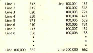
You can do quite a bit with these few commands; we illustrate a "splice." Assume that during one session, a performance was recorded by placing each sample (1/50,000 of a second) in each line of a file called "Performance 1" as follows:

Line 1 312

Line 2 715

Line 3 020

Line 4 358

Line 5 971

Line 6 210

Line 7 713

Line 8 358

Other data not shown

Line 100,000 382

I.e., we stored two seconds of music (100,000 samples); the line numbers do not actually appear in the file (they are assumed or available on request); the numbers represent, as it should be clear by now, the height of the sound wave at time 1/50,000, 2/50,000, etc. (They should really be written in binary code, but we use decimal notation for clarity.)

----------------------

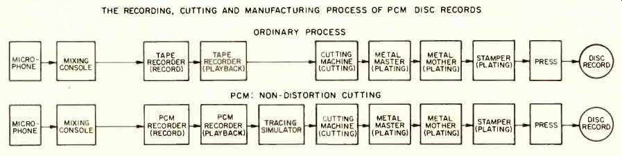
Fig. 14--The Denon system. THE RECORDING, CUTTING AND MANUFACTURING PROCESS OF PCM DISC RECORDS

Electrical Performance and Features

1) Wide dynamic range (more than 89 dB in practical use).

2) Low distortion factor (less than 0.1 percent at operating level).

3) No wow and flutter (not measurable).

4) No interchannel crosstalk (less than-80 dB).

5) Flat frequency characteristic over a wide range (D.C. to 19 kHz, ±0.2 dB; d.c. to 20 kHz, +0.2,-1.0 dB or less).

6) No modulation distortion.

7) Multi-channel recording and playback (2, 4, and 8 channels).

8) Capable of half-speed reproduction, i.e., capable of increasing cutting capacity sharply (characteristic at half-speed playback; d.c. to 10 kHz, ±0.5 dB or less).

9) Equipped with an advanced head (2 channel, direct recording, for variable pitch, which makes cutting as efficient as in the case of conventional records).

10) Capable of editing and splicing.

11) Little loss in duplication.

12) No ghost, can be stored for a long time.

Outline

1) Configuration--PCM converter, 4-head low-band VTR, audio and waveform monitor.

2) Specifications:

a) Modulation--Pulse code modulation, 14-bit sign and magnitude binary code.

b) Transmission clock frequency-7.1825 MHz.

c) Transmission waveform--Standard TV signal (except vertical synchronizing signal).

d) Audio sampling frequency--47.25 kHz.

e) Number of audio channels--2, 4, 8, selectable.

f) Advanced signal recording method--Direct recording.

g) Number of advanced signal channels--2.

h) Magnetic tape recorder used--4-head low-band VTR.

i) Tape speed-38 cm/S.

j) Head-tape relative speed--40 m/S.

k) Acceptable tape--two-inch video tape.

--------------------------

Assume that a second performance of the same musical piece was saved in a file called "Performance 2" as follows:

Other data not shown

Line 100,000 662

Finally, assume that we would like to keep the first 6/ 50,000 of a second from Performance 1 and the rest from Performance 2. The commands are:

Read Performance 1.

Merge Performance 2.

Delete 7, 100,006.

Save Mastertape.

And there is your tape splice. What we did was to bring the first performance in and add on the second performance to get:

Next, by deleting (that is deleting electronically or erasing that part of the memory, or asking the computer to forget something) from Lines 7 to 100,006 we obtain:

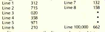
The editor re-sequences the line numbers to obtain a contiguous set of data. Finally, we save the new product into a file called "Mastertape." As you may be aware, special equipment is needed by the recording companies to carry out the mixing process; this is indeed the area where the first big steps forward in the introduction of digital audio equipment have occurred. At the 1978 Convention of the Audio Engineering Society, for example, many manufacturers introduced editing mastering systems and other equipment. Sony introduced the PCM-1600, a 16-bit two-channel PCM processor to be used with video cassette recorders; with the PCM-1600 a studio can record a stereo master or sub-master with 90-dB range and less than 0.05 percent distortion. Wow and flutter are immeasurable, being functions not of the mechanics of tape transport but of a quartz sampling rate clock. An all-digital mixer, a digital reverberator unit, a multi-channel digital recorder, and precise A/D-D/A converters were also presented. Other manufacturers (notably 3M) displayed a similar range of equipment [7]. For a current view of what is available at the consumer level, consult [1].

Digital techniques can not only be used to produce excel lent recordings, but also to allow the revitalization and restoration of old recordings, by a process developed by Thomas Stockham to filter out some type of noise which plagues such recordings [8].

Elementary Signal Processing Devices Digital delay units now widely available are in effect elementary signal processing devices; we call them simple since no complex operations (as Fast Fourier transforms, spectrum evaluation, digital filtering) are performed; a digital noise suppression device would, on the other hand, be considered a full-fledged signal processing system. Below, we briefly describe the operation principle of two well-known delay units:

The Advent 500 and Audio Pulse Model 2 (based on [9]).

The circuitry of the Advent Model 500 SoundSpace control uses eight random access memories (RAMS) with 4,096 bits each. Incoming audio signals pass through a variable gain buffer amplifier and are then filtered into low- and high-pass segments. The low-frequency signals are sampled every 62.5 NS; this corresponds to 16,000 samples per second or a bandwidth of 8 kHz. Each sample is converted into a 10-bit representation using a floating-point technique that provides up to 80 dB of dynamic range.

Conversion from analog to digital representation takes place in two separate steps. The sample is first sized in 10-dB steps, thereby determining the value of the two floating point bits. The remainder of the sample is then compared to a linear ramp, and eight bits of continuous digitization are derived. The combined 10-bit representation is stored in a random access memory and will be recalled when needed by the 10-MHz, quartz-crystal clock-controlled logic. At the appropriate time, each sample is retrieved from memory and reconverted into the analog equivalent by an operation which is the reciprocal of the digitalization system.

The delay value, selected by altering the "size" control on the front panel, determines the primary time delay (in milliseconds) for the longest "early reflection." This provides an index for apparent "room size." A single large memory holds discrete information from both left and right channels, each sample having a distinct address. Delayed information is purposely mixed, contoured, and multiply delayed in controlled proportions. Each output channel contains delayed information from its corresponding input plus blended signals from prior times and spatial origins. In effect, each output channel becomes a "time series" corresponding to the sound field of a specific sound space.

The Audio Pulse Model Two time delay unit also includes audio signals in the digital domain, but rather than using PCM, it uses Delta Modulation. Instead of generating coded groups of pulses at regular intervals to represent the amplitude of the audio signals at every moment, Delta Modulation uses a waveform detector to digitally encode the moment-to-moment changes in the audio signal waveform. This system requires a smaller digital memory and lowers the cost of the circuitry required to do the job.

Coding of Speech

Extensive progress has been made over the past 5 to 15 years in digital speech coding. As we have indicated, PCM techniques could be used here (and in fact they are), but PCM is the Cadillac of the coding schemes. First of all, typical telephone lines have a frequency response between 300 Hz and 3 kHz (who knows if it is flat?); hence 64,000 bits per second (8,000 samples at 8 bits per sample) would be sufficient here. However, since we are dealing with a well-defined acoustical mechanism (namely, the human vocal sys tem) we can say that the field is specialized, and many vocoder-like (voice synthesis) techniques can be exploited.

----------

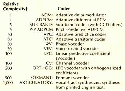
Table II--Vocoder types, based strictly on [5].

Essentially a relative count of logic gates. These numbers are very approximate, and depend upon circuit architecture.

By way of comparison, Log PCM falls in the range of 1 to 5.

------------

Table II, based directly on [5] lists and ranks the various schemes; also see Fig. 15.

The highest quality is achieved by log PCM (at 56,000 bits/ S) and ADPCM (at 32,000 bits/S), both telephone quality, followed by log PCM (at 36,000 bits/S), APC (at 7,200 bits/S), at the communication or speaker identification level, followed by LPC (at 2,400 bits/S) and formant vocoder (at 500 bits/S) which produce synthetic quality speech. Very extensive research is taking place in this area; [5] lists over 100 technical articles and several textbooks.

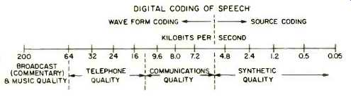
Fig. 15--Spectrum of quality

The goal of a vocoder is to preserve the perceptually significant properties of the waveform with the intention of synthesizing a signal at the receiver that sounds very much like the original. By analyzing the input waveform, or its short term spectra, most vocoders compute parameters that de scribe a simplified model of the speech-production mechanism. Basically, vocoder models assume that speech sounds fall into two distinct classes: Voiced and unvoiced. Voiced sounds occur when the vocal chords vibrate and are characterized by the pitch or rate of vocal chord vibration as well as by the resonant structure of the vocal tract formed from the throat, mouth, and nasal cavities. In unvoiced speech, the vocal chords do not vibrate. Instead, air turbulence, resulting from either the passage of air through a narrow constriction formed by the articulators or the sudden release of air by the lips or tongue, creates acoustic noise that excites the vocal tract. As in voiced speech, the articulators create resonance conditions that, concentrate the unvoiced acoustic energy into particular areas of the frequency-power spectrum. Unlike the voiced case, where energy occurs as discrete frequency components, spectral energy during unvoiced speech is continuous with frequency [3].

In general, the analyzer section of a vocoder determines the resonant structure of the vocal tract, estimates the pitch, and decides whether the speech segment is voiced or unvoiced. The synthesizer section uses these speech features to reconstruct a new time waveform that sounds much like the input. Various vocoders differ in their methods for extracting speech features as well as in their methods for reconstructing speech using these features [3].

The conceptually simplest vocoder is the channel vocoder.

A basic channel vocoder analyzer is shown in Fig. 16. A sequence of bandpass filters is used to divide the voice signal into frequency channels. The signal components in each of the frequency channels are first rectified, usually by a square-law circuit. Then they are either integrated or low-pass filtered, or both, to yield a continuous estimate of the speech power-spectrum amplitude in each channel. Independently of the spectral analysis, a pitch extractor determines the vocal pitch and a voicing detector determines whether the input represents a voiced or unvoiced speech sound [3].

As shown in Fig. 16, the channel vocoder synthesizer re constructs the speech signal using estimates of the power spectrum together with pitch and voicing information. During voiced segments, a pulse generator outputs short pulses at the pitch rate, and these pulses excite a bank of filters similar to those shown in Fig. 7. Each filter output is then adjusted in an attempt to make its energy equal to that measured for the corresponding channel at the analyzer. For unvoiced sounds, a Gaussian noise source excites the filter bank [3].

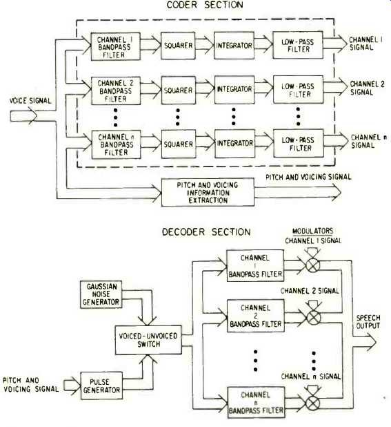
Fig. 16--Channel vocoder.

Summary

In this series of articles, we have examined the principles of digital encoding, a technology which promises to have a major impact on high fidelity in the near future. The theory was developed in the '60s for telecommunications applications, and in the early '70s the first digitally mastered recording was offered commercially. At the current time a range of digitally mastered recordings is on the market; 1980 promises to be the year during which the first fully digital recording and turntable will be available to consumers. After several years of activity in the area of standardization, we should see com pact, inexpensive, reliable, and compatible digital discs of the highest fidelity.

(adapted from Audio magazine, May. 1980)

Prev: Digital Techniques in Sound Reproduction-- Part I (April 1980)

Also see:

Dr. Thomas Stockham on the Future of Digital Recording (Feb. 1980)

Telefunken Digital Mini Disc (June 1981)

= = = =