4.1 BASIC INDUCTANCE AND REACTANCE
Analysis of real inductor and transformer behavior requires a mastery of basic ac-circuit concepts. A condensed treatment of these topics is given in this section and the ones following, both as a review and as a ready reference.
Inductance: If a current is run through a coil of wire, a magnetic field is set up whose strength is proportional to the current and the number of turns. This is the principle of the electromagnet. If a magnetic field is moved through a coil of wire, a voltage is induced across the coil whose magnitude is proportional to the speed of movement and the number of turns. This is the principle of the generator. Figure 4-1(a) and (b) illustrates these effects.
Combining these facts, if ac is passed through a coil, a changing (moving) magnetic field is set up, and this field induces a voltage in the coil that caused it. The direction of this self-induced voltage is always such as to oppose the initially applied voltage. Thus a coil (we call it an inductor-never use one syllable when you can use three) opposes any change in current.
Reactance: Notice that the inductor's opposition to ac is by means of a reverse voltage, not a restriction in the conductive path as in the case of a resistor. We call this kind of opposition reactance as opposed to resistance. The main difference is that reactance does not burn energy-it merely stores it on one quarter-cycle and then bounces it back into the source on the next quarter-cycle.
This bounce-back results in a phase shift between current and voltage for an inductor. Current through the coil reaches a maximum just as the voltage across the coil falls back to zero. We say that current in an inductance lags voltage by 90°.
This is shown in Fig. 4-1(c).
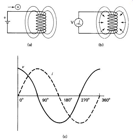
FIGURE 4-1 (a) Current through a coil sets up a magnetic field, (b) Moving
a magnetic field through a coil causes a voltage to be induced across it.
(c) Self-induced voltage causes current to flow back against the direction
of applied voltage from 90° to 180° and again from 270° to 360°.
The amount of reactance that a coil presents to ac depends on the value of the inductance and the speed with which the current alternates (frequency):
X_L=2 pi fL (4-1)
... where XL is the reactance in ohms, f the frequency in hertz, and L the inductance in henrys.
Series and Parallel Reactances: Two inductors in series have a total reactance equal to their sum (just like series resistors), provided that their magnetic fields are not close enough to interact. This is illustrated in Fig. 4-2(a).
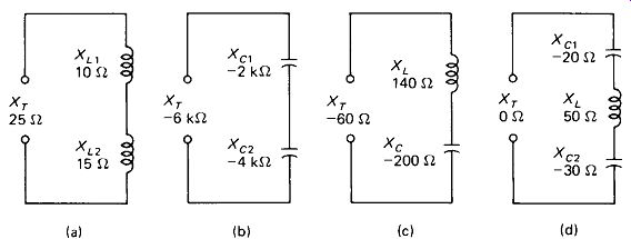
FIGURE
4-2 Reactances series combine by simple algebraic addition, with capacitive
reactance considered negative.
Capacitors store energy in an electric field, and when connected to an ac source, simply bounce this energy back to the source on alternate quarter-cycles.
Thus they present a reactance to ac, much like an inductor. However, there are two important differences. First, the current in a capacitance leads the voltage by 90°; just the opposite of the inductor. We give a negative sign to the reactance of a capacitor:
XC 2-pi fC where C is the value of the capacitance in farads.
Second, as shown by equation 4-2, capacitive reactance varies inversely with frequency f, and capacitance C, again just the opposite of the inductor. This means that as frequency increases, inductive reactance goes up while capacitive reactance goes down. Calculations involving reactances are, therefore, valid only at the frequency for which reactance has been calculated. Capacitive and inductive reactances in series are subtractive, as illustrated in Fig. 4-2(c) and (d).
Reactances in parallel are governed by the same formulas as resistors, namely, the product over the sum and the reciprocal of the reciprocals. In this case, however, attention must be paid to the signs. Figure 4-3 gives some examples.
4.2 BASIC CONCEPTS OF IMPEDANCE
Series Resistance and Reactance: When resistance and reactance are placed in series, the result is termed impedance. Part of the energy delivered by the source is then dissipated as heat (in the resistance) and part is reflected back to the source (by the reactance). Current will lag applied voltage if the net reactance is inductive, and lead if the net reactance is capacitive, but by an angle between zero and 90°.
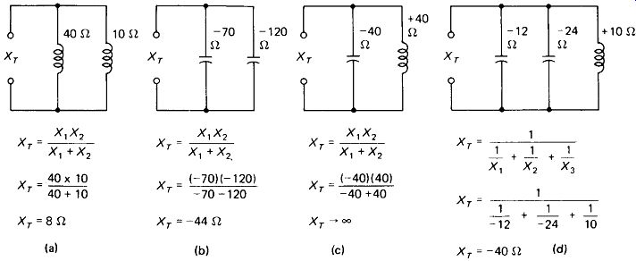
FIGURE 4-3 Reactances in parallel combine by the product over the sum or
the reciprocal of the reciprocals as do resistors. Again, capacitive reactance
Is negative.
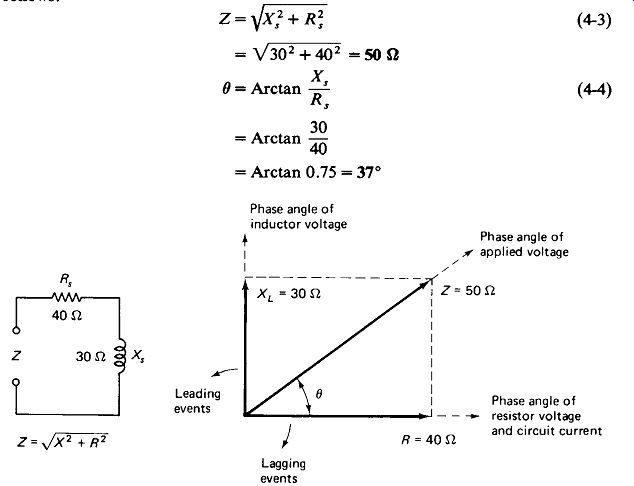
FIGURE 4-4 Resistance and reactance cannot be added or subtracted directly.
The combination, called impedance (Z). is obtained by phasor addition.
The total value of the impedance Z and the exact phase angle 9 are determined by phasor addition of X and R, as shown in Fig. 4-4. The calculations proceed as follows:

(4-3)
Notice that the total circuit current is in phase with the resistor voltage and lags the applied voltage by 37°.
A few trial calculations with equation 4-3 will show that, if Xs is three times Ra or more, the total impedance is only 5% greater than Xs. Likewise, if Rs > 3XS, Z is greater than Rs by only 5%. We will often find it helpful to neglect the lower of Xs or Rs in these cases, so ZmRs if Xs is small, or ZsmX3 if Rs is small.
Parallel Resistance and Reactance: When resistance and reactance appear in parallel, the equivalent impedance is always less than the smaller of the two, but never smaller than 0.707 times the lower one. The phase shift is characteristic of the reactance involved: total current lagging applied voltage for inductance, leading for capacitance. The exact impedance and phase angle can be calculated:

(4-6)
In the parallel circuit it can be shown that, if Xp is at least three times Rp (or vice versa), the impedance of the parallel combination is less than the lower value (Xp or Rp) by only 5%. Here, again, we will often find it appropriate and helpful to disregard the higher parallel value (Xp or Rp ), so ZmXp if Rp is large, or ZznRp if Xp is large. Such simplifications can be of great help in analyzing real inductor and transformer equivalent circuits. A few examples are given in Fig. 4-5.
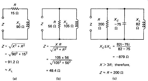
FIGURE 4-5 (a) Series resistance Is negligible if reactance is three or
more times larger, (b) Equation 4-5 always gives parallel impedance lower
than the smaller of X or R. (c) The parallel reactances are combined first,
giving a net reactance much larger than R, so that Z«Xp.
The exact Z, by equation 4-5, Is 195 ohm.
Equivalent Series and Parallel Circuits: Any parallel R-X circuit can be replaced by an equivalent series R-X circuit using the following equations:
R=X„ X=Rr Xp Rp , X? + R>p X p Rp
Conversely, any series R-X circuit can be replaced by an equivalent parallel circuit using the equations:

(4-10)
Of course, these equivalencies are valid only at the particular frequency for which the reactance has been calculated. Also note that all of the reactances are to be placed into these formulas as absolute (unsigned) quantities. Although capacitive reactance has been termed negative, it can be subtracted only from inductive reactance ( XL - Xc valid), not from resistance (R - Xc invalid).
Using the reactance combination methods illustrated in Figs. 4-2 and 4-3 and the equivalency formulas 4-7 through 4-10, it is possible to reduce most circuits containing numerous R, XL, and Xc components to a single series or parallel R-X equivalent.
EXAMPLE 4-1
Figure 4-6(a) shows a series-parallel RLC circuit. It happens to represent a real transformer, but we’ll get to that later. For now, determine the power delivered to R2, which represents the load.
Solution
First it is necessary to calculate the reactances:
-663 a XL2 and Xc can be parallel-combined:
+i5AQ Xli + Xc 75.4 - 663
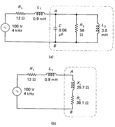
FIGURE 4-6 Circuit for Example 4-1, illustrating parallel-to series X-R
conversion to obtain a solution: (a) initial trans former representation;
(b) reduced to a simple series equivalent.
Now the parallel combination of R2 and Xp can be converted to its series equivalent:
The equivalent circuit now stands as in Fig. 4-6(b), and consists of a total series resistance and inductive reactance:
RsT=Ri +Rs= 12 + 39.1 =51.1 ohm X,t
= Xli +XS- 22.6 + 25.7 = 48.3 l ZT = Jx?T+ R1,t = V48.32 + 51.12 =70.3 ohm
The total current is …
This current a flows through the impedance of C, R2, and L2 in parallel, producing a voltage across R2:
4.3 BASIC RESONANCE CONCEPTS
This section discusses the effects of resonance and tuned circuits. After that we we’ll be equipped to start talking about real inductors.
Series Resonance: You may have noticed that in the example of Fig. 4-2(d), the inductive and capacitive reactances exactly canceled, leaving a net reactance of zero. This short-circuit condition prevails at only one frequency, called the resonant frequency, which is given by ...
[4-11]
... is in hertz, L is in henrys, and C is in farads. At lower frequencies the capacitive reactance predominates and at higher frequencies the inductive reactance predominates. We therefore have a series tuned circuit which can be placed in series with a line to pass only the resonant frequency or in shunt across the line to trap out the resonant frequency.
Series Circuit Q: Of course, the series tuned circuit is not a perfect short circuit at resonance. The coil has some resistance, perhaps increased by the skin effect (Section 1.4) if the frequency is high, and at very high frequencies the capacitor may have an appreciable dissipation factor, which can be represented as additional series resistance according to equation 3-4. The ratio of the reactance of either the coil or the capacitor at resonance to the total effective series resistance is termed the quality factor or Q of the series tuned circuit:
… at resonance (4-12)
When a series tuned circuit is used in series with a load resistance and / or a source resistance, the entire series resistance must be included as Rs in determining Q.
This is illustrated in Fig. 4-7(a).
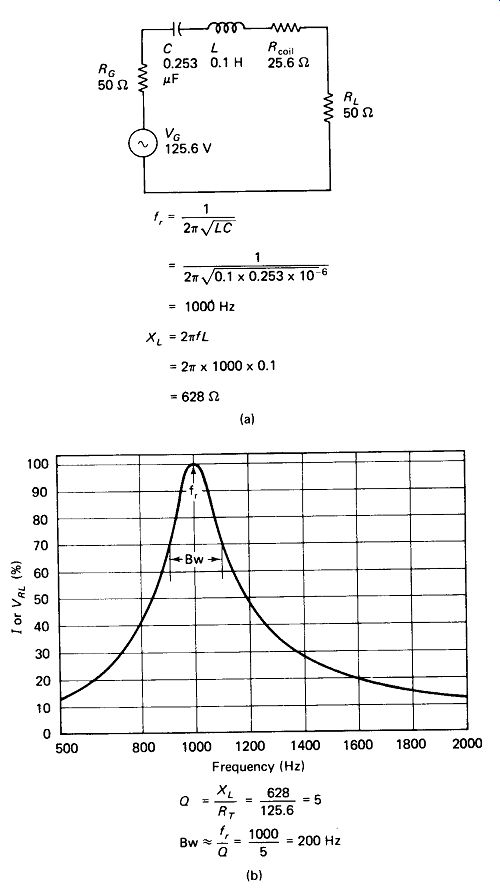
FIGURE 4-7 Q (quality) of a series-tuned circuit is defined as X/R, where
X is either Xc or XL (equal at resonance) and Ft is the total resistance
in series at resonance: (a) the resonant circuit; (b) response at frequencies
off resonance.
Bandwidth Bw is defined as the span between the -3dB (0.707 voltage) points.
Bandwidth: The current through a series tuned circuit is maximum at resonance, and decreases above or below that frequency as net inductive or capacitive reactance appears in the circuit. Series-circuit analysis, as illustrated in Fig. 4-4, can be used to determine the current response at any frequency, and a graph of the results appears in Fig. 4-7(b). Of particular interest are the frequencies at which the response falls by 3 dB (to 0.707 of maximum). These are commonly termed the lower (f1) and upper (f2) cutoff frequencies or half-power points. The frequency span between them is called the bandwidth and is approximated by
Bw = f_r/Q (4-13)
The approximation grows better as Q goes higher, being about 5% off when Q = 5.
Bandwidth is easy to measure experimentally, and narrow bandwidth (high (?) is generally a desirable feature in a tuned circuit. At frequencies beyond f1 and f2, the response can be determined from the following table:
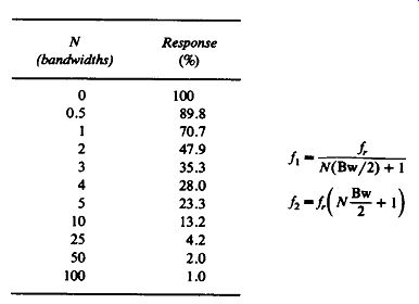
------
Voltage Rise at Resonance: Notice that in the circuit of Fig. 4-7(a) the total impedance seen by the source at resonance is 125.6 Q purely resistive, and the current is
V/R = 126.5 V / 126.5 ohm =1 A.
This current flows through Xc and XL, producing voltages across each of them, even though their reactances cancel. The voltages produced are:
VXL = Vxc = IXc = 1 A X 628 =628 V
These voltages are larger than the source voltage by exactly a factor of Q (five times in this case). In general,
Vxl=Vxc=QVc (4-14)
… for a series-resonant circuit, where VG is the open-circuit generator voltage and Q is calculated using the entire circuit resistance. Notice that with Q = 50 and VG = 100 V, the voltage rating required of the capacitor becomes 5000 V. This is no idle theory! The voltage rise at resonance must be considered when selecting components for series-resonant circuits.
Of course, since VXL leads the circuit current by 90° and Vxc lags by 90°, the two voltages are 180° out of phase and exactly cancel each other. Thus the voltages across the circuit elements Rc, C, L, Rc, and RL in Fig. 4-7(a) add up to 125.6 V, which is the generator voltage.
Parallel Resonance: In the circuit of Fig. 4-3(c), equal capacitive and inductive reactances were placed in parallel, and the resulting reactance rose to infinity. This was because the two currents (IL = V/XL and Ic = V/Xc) were equal and exactly 180° out of phase, resulting in zero total current. Figure 4-8(a) shows a real parallel-resonant circuit with the inevitable series resistance of the inductor. Equations 4-9 and 4-10 can be used to change Ls and Rs to their parallel equivalent, but if Q is reasonably high, we can operate with the much simpler approximations:
(4-15) (4-16)
The error incurred with Q_coil
= 5 is 4%, dropping to 1% at Q = 10.
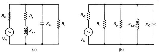
FIGURE 4-8 Parallel tuned circuit: (a) as found in practice with generator,
load, and series coil resistances; (b) equivalent with all resistances appearing
in parallel.
Qp -Rp(tot)/Xp.
The Q of the entire circuit can now be determined from the equivalent circuit of Fig. 4-8(b) with Rc, RL, and Rp appearing in parallel:
The maximum output voltage at resonance is:
(4-18)
The curve of Fig. 4-7(b) can be used to determine the output at other frequencies.
Notice that on high-impedance lines (Rc and RL above 100 i or so) the highest Q is obtained with a parallel-resonant circuit across the line, while low impedance lines are more sharply tuned with a series-tuned circuit in series with the line. Also notice that with the parallel circuit, a low L/C ratio (small inductance, large capacitance) will produce lower reactances at resonance, and hence higher Q, according to equation 4-17, while the series circuit will tune more sharply with a high L/C ratio, according to equation 4-12. Some of the advantage of increasing L in the series circuit is offset by the inevitable increase in Rs of the coil when its number of turns increases. However, L increases by the square of the turns, while Rs increases linearly, so substantial benefits may be realized.
Resonant Traps: Figure 4-9(a) and (b) show, respectively, a series-resonant trap across the line and a parallel-resonant trap in the line, together with formulas for their Q and minimum output at the null point. Again, these formulas are approximations whose accuracy falls off markedly below a Q of 5. It is also assumed that Rs is much less than either Rc or RL. Notice that the depth of the null is completely dependent upon Rs, whereas the sharpness of the null is dependent upon the ratio of reactance at resonance to line impedance. As with the peaking tuned circuits, series-resonant traps tune most sharply with a high L/C ratio on a low-impedance line, whereas parallel-resonant traps have highest Q with a low L/C ratio on a high-impedance line.
EXAMPLE 4-2
Design a tuning circuit with a - 3 dB passband from 110 to 140 kHz. The source resistance is 40 k-Ohm and the load impedance is essentially infinite. A 2.5-mH coil with a Q of 8.0 at 125 kHz is available.
Solution Solving equation 4-11 for C gives the required capacitance:
The Q required if the parallel-resonant circuit of Fig. 4-8(a) is used is obtained from equation 4-13:
= 4.17
FIGURE 4-9 Resonant traps: (a) series tuned across the line; (b) parallel tuned in series with the line; (c) response curve showing bandwidth and null depth.
The parallel resistance needed to produce this is obtained by equation 4-17:
XL - 2 pi fL= 1960 ohm
Rp = QX = 4.
17 X 1960 = 8.17 k Ohm
The coil's series resistance and its parallel equivalent, by equation* 4-12 and 4-16, are:
The effective parallel resistance of Rc and Rp is 40 k ohm || 15.68 k ohm, or 11.26 k Ohm. A shunt resistance, sufficient to bring the parallel total down to the necessary 8.
17 k ohm, must now be added in the R L position of Fig. 4-8(a). The value is calculated by the product over the difference:
The practice of shunting a tuned circuit to lower its Q and widen the bandwidth is in common use.
4.4 REAL INDUCTORS
For the sake of discussion and analysis we will place inductors into four categories, all of which are shown in Fig. 4-10.
Air-Core Solenoid-Wound Coils: These may commonly range in value from 0.1 uH to several mH, having one to several hundred turns. They may be self-supporting in air, or wound on a ceramic, plastic, or cardboard form. Their diameter depends upon inductance required and power level, but commonly ranges from 0.5 to 5 cm, with still larger sizes appearing in high-power transmitters. When used in frequency-sensitive tuning and filtering circuits, they are called coils, and their exact inductance and its stability are likely to be critical. When used simply to block high frequencies they are called rf chokes, and wider tolerances and lower Q, s are generally acceptable.
Coils with Open-Path Magnetic Cores: These are wound on forms commonly between 0.5 and 2 cm in diameter, and have powdered iron or metal oxides (ferrites) in the core to increase the inductance. The core may be an adjustable slug on screw threads, providing variable inductance. Their values range to a few hundred millihenrys.
Coils with Closed-Path Magnetic Cores: These are wound on a form consisting of strips (laminations) of iron, as shown in Fig. 4-14, and are often enclosed (potted) in a steel cover. They contain several hundred to several thousand turns of wire, and common values range from a few millihenrys to several hundred henrys.
Common sizes are from 2 to 10 cm on a side, although much larger units are available for high-power applications. They are generally used to block the flow of relatively low-frequency ac (either audio or line-frequency ripple in a power supply) while passing dc. Tolerance is generally rather broad ( - 20, + 50% typical) and Q is relatively low. They can be designed with an adjustable air gap in the core to provide variable inductance.
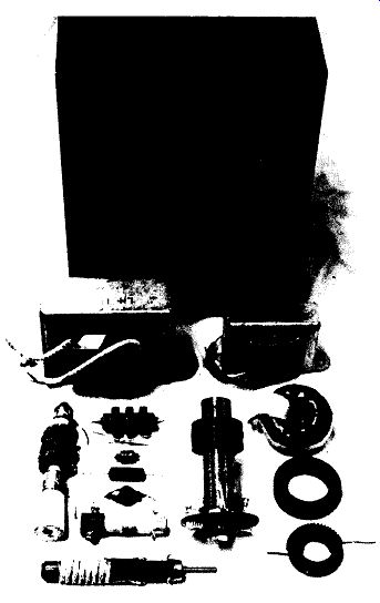
FIGURE 4-10 Representative inductors. Top: large potted power-supply choke
with two smaller lower-current 0.5-H open-frame units below, all wound on
E-l laminated iron cores; left: 2.5-mH and 1-mH air core RF chokes, with
small 1.8-mH ferrite-core choke below, followed by 6.8-/iH and 100-fiH air-core
chokes, and two ferrite slug-tuned coils; center: ferrite-slug-adjustable
inductor of 20 mH; right: three toroids, 70 mH coated, blank core, and 1.8
mH wound of AWG 18 wire.
Toroidal Inductors: Toroids are wound on donut-shaped cores of magnetic materials specially formulated for temperature stability, low loss, and high permeability. Nonmagnetic cores may be used for microhenry values. Because the turns cannot be wound on a simple rotating drum or bobbin, toroids are considerably more expensive than af chokes of equal inductance. However, by proper selection of core material and winding, they can achieve a remarkably high Q, often above 100 in the frequency range 1 kHz to 1 MHz. Their tolerance, linearity, temperature stability, and Q are generally far superior to inductors wound on laminated iron cores.
Predicting Inductance: The inductance of an air-core coil of known dimensions can be predicted to within about 10% by the formula
[4-19]
where L is in micro-henries, d is diameter in centimeters, l is length in centimeters, and N is the number of turns. The equivalent with d and l in inches is
(4-20)
Figure 4-11 illustrates the application of the formula. The formula is most accurate for single layer coils of 10 turns or more, but is still useful for smaller or multilayer coils. For iron-or ferrite-core coils, be sure to see Section 4.6 on core effects.
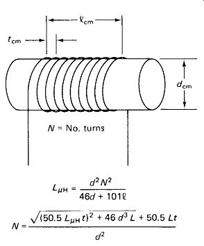
FIGURE 4-11 The Inductance L or turns required N for an air-core coil diameter
d and length I.
Turn spacing center to center is designated t.
Usually, the question is not "calculate the inductance of a given coil, "but rather " wind me a coil of a given value."
Solving the foregoing equations for N with tN substituted for /, gives the somewhat unwieldy turns-winding formula for single-layer close-wound coils:
(4-21)
where N is the number of turns required, L is the desired inductance in microhenries, d is coil diameter in centimeters, and t is the wire thickness (including insulation) in centimeters. The same formula, with d and t in inches, becomes:
(4-22)
For multilayer coils wound on a bobbin of a given length, the required number of turns is given by direct transposition of equations 4-19 and 4-20:
(4-23)
(4-24)
Stray Capacitance and Resonance: Adjacent turns of wire in a coil have a certain amount of capacitance between them, the total effect being very much as if a single capacitor were placed across an ideal inductor, as in Fig. 4-12(a). This, of course, gives the coil a natural parallel-resonant frequency, above which its reactance is capacitive and decreases with frequency. Using a coil at one-fifth of its resonant frequency will result in an apparent inductance increase of 4%. At one-third the resonant frequency the increase is 11%, and at 0.5 fr it is 25%. The coil is still useful as a choke up to and beyond parallel resonance, however, since its impedance is still very high.
As frequency is increased above the parallel-resonant point, the impedance (capacitive) of the coil will drop until a point is reached at which the stray capacitance from the bulk of the coil becomes series-resonant with the first turn or so on the end of the coil. Impedance at this natural series-resonant frequency drops to near zero as shown in Fig. 4-12(b). There may be several more series-resonant points above the first one, but the coil is useless even as a choke above the first one. When a wide range of frequencies is to be blocked, two chokes in series may be used. The first, placed at the "hot" end, is small and has a very high series-resonant point. The second, placed at the "cold" or ac ground end, is large and has its series-resonant point at a frequency where the reactance of the first choke is high.
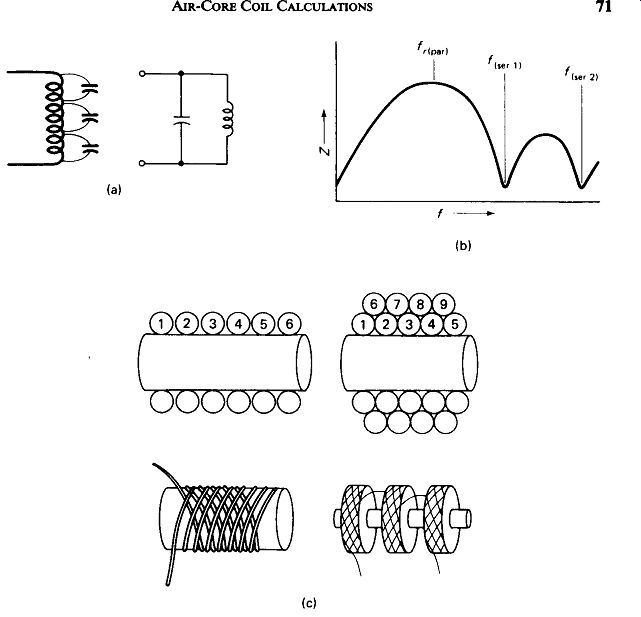
FIGURE 4-12 (a) Stray capacitance between turns gives a colt a natural parallel-resonant
frequency, (b) Impedance of a coil versus frequency showing parallel-resonant
and (higher) series-resonant frequencies, (c) Four methods for reducing stray
capacitance in a coil (see the text).
A grid-dip meter coupled to the open-circuited coil will detect the parallel resonant point. With the terminals shorted, the dip meter will respond to the series-resonant points. The shorting wire may have to be looped once around the dip meter's coil to provide adequate coupling. Figure 4-12(c) shows four techniques for reducing stray capacitance and hence raising the natural resonant frequency of a coil. The first is simply to keep the turns spaced apart, since capacitance varies inversely with conductor spacing. Of course, this spacing also decreases the inductance by increasing length (see equation 4-19), but if the spacing is limited to one-half the wire diameter or less, significant improvement can be realized.
Spacing can be achieved by using specially grooved forms, by winding a string along with the wire to hold the space, or by simply using Teflon-insulated wire in place of the usual thin enamel insulation. Common PVC (polyvinyl chloride) insulated hookup wire should never be used for winding coils. PVC has severe dielectric loss at certain frequencies which are a function of temperature, and serious reduction in the Q of the coil will result. Bakelite coil forms should be avoided at radio frequencies for similar reasons.
The other techniques for raising f_s illustrated in Fig. 4-12(c) are (2) keep the starting and finishing coils of a two-layer coil at opposite ends of the form, (3) use a diagonal-pitched winding, alternating direction with each layer so the wires are close only at the crossing points, and (4) wind the coil in separate sections (called pies), and build up the required inductance by series-connecting the required number of these low-value high-/. coils. This last technique has the drawback of requiring more wire than a single bulk coil because there is no mutual inductance between windings of different sections. The result is higher winding resistance and lower Q.
Estimating the stray capacitance of a coil is difficult because it depends upon so many factors: insulation thickness and dielectric constant, coil spacing, layering, winding pattern, wire thickness, and coil diameter primary among them. However, for single-layer close-wound coils using No. 32 to No. 18 enameled wire on 1- to 3-cm forms, capacitance will generally be in the vicinity of 0.05 pF/turn. Multi layered coils may have less than half that capacitance. Spaced winding and cross-pitch winding can reduce the capacitance by about 25%.
Skin Effects and Q:
In the absence of nearby objects, such as shields or other components, the Q of an air-core coil depends almost entirely on the resistance of the wire at the frequency in question. The formulas for skin-effect resistance of copper wire are therefore reproduced from Section 1:
(1-4)
... where 8 is skin depth in centimeters, t is wire diameter (thickness) and fI is wire length, both in the same units, and / is in hertz. In winding coils for high frequencies it is necessary to consider the proximity effect as explained in Section 1-4.
Some examples from the laboratory will serve to demonstrate the utility of the inductance and skin-effect formulas.
EXAMPLE 4-3
The core was removed from an audio choke. The remaining air winding had an average diameter of 3.0 cm and a length of 2.2 cm, and was wound of wire with a thickness measured as 0.014 cm. The dc resistance of the coil was 460 ohm. Predict the coils inductance and Q at 1000 Hz.
Solution
Interpolating from the wire table (Fig. 1-1), this wire has a resistance of about 0.011 ohm/cm. The resistance of one turn is then
= 3.14 X 3 X 0.011 - 0.104 ohm
The number of turns is then found from the total resistance:
N = 4420 turns
R1 0.104 The inductance, from equation 4-19, is
_
32 X 44202 _0j 4lBH 46d+ 101/ (46 x 3) + (101 x 2.
2)
The skin depth at 1000 Hz is calculated from equation 1-3:
= 0.21 cm
This is 30 times the radius of the wire, so skin effect is negligible and the dc resistance is used:
_ X 2-nfL 6.28 X 1000 X 0.488 , _ V = R=R-460- f f7
The inductance and Q of the actual coil, as measured on a commercial bridge at 1000 Hz, were 0.47 H and 6.6, respectively.
EXAMPLE 4-4
Find the inductance and Q at 3 MHz of a 30-turn close-wound coil of No. 22 enameled wire on a 1.9-cm-diameter plastic form.
Solution:
The thickness of the wire, from the table in Fig. 1-1, is 0.064 cm. Allowing 0.002 cm for the enamel, the length occupied by 30 turns is calculated:
l = Nt = 30 X 0.068 - 2.04 cm
The inductance, from equation 4-19, ...
The skin depth, by equation 1-3, is ...
This is 84 times less than the wire radius, so the skin-effect resistance is calculated by equation 1-4:
Wire length= lw
[...]
Checking the table in Section 1-4, we make a not-too-confident estimate of the proximity-effect resistance as ten times the calculated skin-effect resistance, or 4 ohm.
The measured values for L and Q of the actual coil at 3 MHz were 9.6 /tH and 41, respectively.
---------------
FIGURE 4-13 Actual reactance, resistance, and Q for a 1-mH air-core three-pie cross-pitch choke. R holds at its dc value until skin effect causes it to rise as Vf . X increases as f until parallel resonance (9 MHz) brings it up and series resonance (35 MHz) brings it down. Q rises as f until skin effect begins, whereupon Q rises as Vf until parallel resonance, where it is maximum. Above f, the 1-mH coil becomes swamped by the stray effects and is no longer accessible. Q readings above fr therefore apply to the stray effects and not to the coil as such.
-------------------
The Q of a coil is not a constant, but varies with frequency in a generally predictable way, as shown in Fig. 4-13. At low frequencies, XL is low, although the resistance of the wire is equal to its dc value. Q is therefore relatively low. Q increases linearly with frequency until the skin effect begins to raise the value of R.
Since XL goes up as /, while R goes up only as V/ . Q now rises as V?:
Q = - cc -- = Vf R Vf
At the self-resonant frequency, Q is supposedly at a maximum, since the reactance of XL and Xc in parallel approaches infinity. However, the coil is not purely inductive at this point. The maximum usable Q should generally be read at 0.5 to 1/5 the frequency of the peak at fr.
4.6 MAGNETIC-CORE INDUCTORS
Core Effect on Inductance: A magnetic field can pass much more readily through a magnetic metal such as iron or nickel than through air. This fact is demonstrated by the common tick of holding up a sting of a dozen straight pins from a single magnet at the top. We say that the magnetic metals have a higher permeability than air. To the extent that we can provide a high-permeability medium within and around a coil, we can increase its inductance for a given number of turns. Although the amount of increase depends upon the exact shape and composition of the core, we can estimate that a slug of magnetic material in the center of the coil will provide an inductance increase of seven times over an air core. Brass slugs are occasionally used in rf coils to provide an inductance decrease of up to 25%.
Calculating Core Effects: The highest inductances are obtained by providing a complete magnetic flux path through and around the coil. Figure 4-14 shows the common methods for achieving this. The CI- and El-shaped stacks of silicon-iron strips insulated with varnish have long been popular and still prevail at power-line and audio frequencies, while the newer ferrite materials in the pot core and toroid ring structures generally offer superior performance in the ranges above a few kilohertz.
The inductance of a cored coil with no air gap can be calculated with reasonable accuracy from the formula:
(4-25)
where N is the number of turns, n the relative permeability of the material, A the cross-sectional area of the core in cm^2 , and I the effective magnetic path length in centimeters. Note that in the E-I structure there are two parallel paths if the coil is wound on the center post, so the effective length is:
WX + [XZ + ZY+ YW] / 2
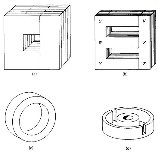
FIGURE 4-14 Popular magnetic-core configurations: (a) alternating layers
of C-l-shaped silicon-iron strips; (b) the more popular E-l-shaped laminated
core; (c) toroid core of ferrite material; (d) ferrite pot core (one of two
identical halves); coil is wound on a plastic bobbin and slipped over center
post.
For the pot-core structure, the effective length and area are generally given by the manufacturer.
Air-Gap Considerations: All of the structures in Fig. 4-14 except the toroid contain an air gap in the flux path. It may be less than 0.01 cm, due primarily to the insulating varnish coat on the laminations; or it may be intentionally made much larger, or made variable to allow adjusting inductance. The inductance of a coil having a magnetic core with an air gap can be calculated from ...
(4-26)
... where l_g is the length of the gap in centimeters, L_c the effective core length in centimeters, and the other terms are as above. Values of u for various popular core materials are given in the table of Fig. 4-15.
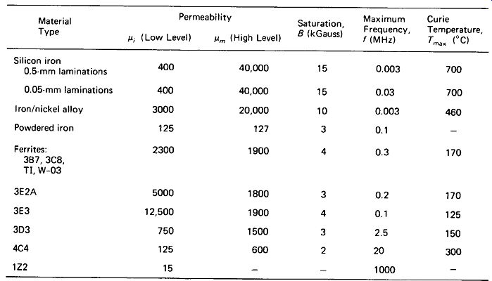
FIGURE 4-15 Properties of common magnetic-core materials.
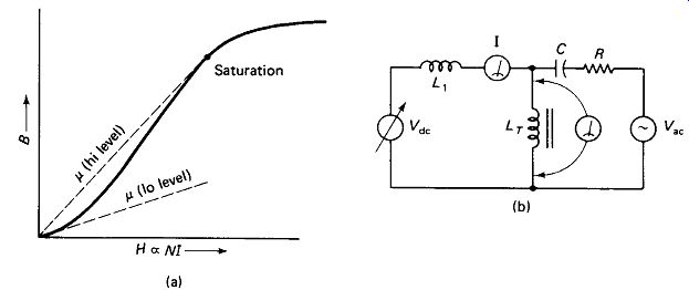
FIGURE 4-16 (a) Magnetic flux density B versus magnetizing force H for a
typical magnetic material. Initial permeability u , is generally lower
than maximum-level permeability u_m. (b) Circuit for measuring the dc saturation
current of an inductor.
Besides lowering the inductance, the presence of an air gap has the important effect of linearizing the core. Notice from Fig. 4-15 that for most materials p varies markedly from low- to high-level magnetization. This is further illustrated in the magnetization curve of Fig. 4-16(a). The air gap adds a constant and relatively large reluctance (the magnetic equivalent of resistance) to the magnetic path, tending to swamp out the reluctance changes of the core material. Nevertheless, it is common to find that an iron-core inductor measures 1 H at low signal levels and 2 H at higher levels. Waveform distortion can also be expected due to the nonlinear response of magnetic-core inductors.
Core Saturation: There is a limit to the degree of magnetization (molecular alignment) that a material can obtain, and this places a limit on the peak current that can pass through a magnetic-core coil without causing saturation. If this limit is exceeded with ac, the coil suddenly stops generating inductive reactance to the ac and becomes (almost) a simple piece of wire. The result could be excessive current, overheating, and the destruction of the coil.
The slope of the magnetization curve, Fig. 4-16(a), equals permeability, which is proportional to inductance. Notice that this slope drops to near zero as current I is increased. The value of flux density B in the core of an ac-excited coil can be calculated from
B =- - (4-27)
... where B is in gauss, V is in volts, f is in hertz, N is turns, and A is the cross-sectional area in cm^2.
Notice that u and l do not enter this equation, since their effect on flux density via reluctance is exactly offset by a reciprocal effect on current via inductance. The value of B must be kept less than the saturation value given in Fig. 4-15.
The flux density for a dc-excited coil is 1.
267V/ t . + Uv (4-28)
where B is in gauss, N is turns, / is dc amperes, tg is air-gap length in centimeters, lc is effective core length, and u is core permeability.
EXAMPLE 4-5
An inductor is wound on a C-I-shaped core of silicon-iron laminations. The legs of the lamination stack are 2 cm wide by 2 cm thick, and the overall dimensions of the core are 6 cm X 6 cm. An air gap of 0.05 cm is left in the core. The winding consists of 900 turns of AWG 24 enameled wire. Calculate the inductance at high and low excitation levels, and determine the maximum dc current before saturation.
Solution
Low-level n is 400, high-level n is 40,000, lc is 4 x 4 or 16 cm, and A is 4 cm^2. Using equation 4-26, we obtain ...
Transposing equation 4-28 to find current for the 15,000-G saturation level yields [...]
Measuring Saturation: Figure 4- 16(b) shows an experimental circuit for measuring the dc saturation current of a choke. LT is the inductor under test, and the saturation current is measured on dc ammeter I. R must have a value of at least 3 X_lt and Xc must be 1/3 XLT or less. L1 must have a higher current rating than LT and XL1 must be 3XLT or more. L1 can be replaced by a resistor if these conditions are met. In operation, Vac is set to produce a small voltage, say 1 V rms, across L_T. Vdc is then increased until the measured ac voltage drops by a specified amount (usually 10%), indicating that has dropped by 10%.
Useful Saturation: Core saturation can be used to advantage in some applications.
A swinging choke in a power supply is designed to saturate at maximum dc load current. The resulting decrease in inductance allows more charging current to reach the first filter capacitor, thus largely offsetting the output voltage drop under heavy load.
The magnetic amplifier uses a relatively small dc current through a many-turn coil to saturate a core upon which is wound an inductor carrying a heavy ac current. A small increase in the dc can thus cause a large increase in the ac.
Core Effect on Q: The type of core material used in an inductor must be selected for the frequency range of intended use. Thin strips (laminations) of silicon iron are used at power-line and audio frequencies, with powdered iron, and then various compositions of metal oxides (ferrites) being preferred at progressively higher frequencies. The reason for the frequency dependence of the core is this: In magnetizing the core with ac, we are requiring the molecules of the core material to realign their positions every half-cycle. It takes a rather specially composed material to follow these realignments into the high kilohertz and megahertz ranges, and there is always some frictional loss (due to hysteresis) in the process. The Q of a magnetically cored coil is therefore likely to be higher than its air-core counterpart because of its higher XL, but only up to the maximum frequency of the core material, beyond which Q drops sharply due to hysteresis loss.
Predicting Q for a magnetic-core coil is quite difficult, since permeability and hysteresis vary with frequency and material composition. Measurement at the intended frequency is the most practical recourse.