5.1 THE IDEAL TRANSFORMER
The Basic Idea: If two strands of wire are used to wind two coils simultaneously on the same form, a transformer is produced. This is illustrated in Fig. 5-1(a). If an ac voltage is impressed across one of these windings, which is then called the primary, an ac current will flow in the amount IP = VG/XP, where Xp is the reactance of the primary coil at the generator frequency. Since the reactance is inductive, the current, and hence the strength of the magnetic field produced, will lag the applied voltage by 90°, as shown in Fig. 5- 1(b). The other winding, called the secondary, experiences fully the effects of this changing magnetic field, and a voltage is induced in it which is proportional to the rate of change of that field. For a sine-wave input, this rate of change turns out to be another sine wave, which is exactly in phase with the input, as shown in Fig. 5- 1(b). If the number of turns on the primary exactly equals the number of turns on the secondary (NP = Ns), and if the windings are kept perfectly close together so that all of the magnetic field produced by the primary reaches the secondary, the secondary voltage will be an exact reproduction of the primary voltage.
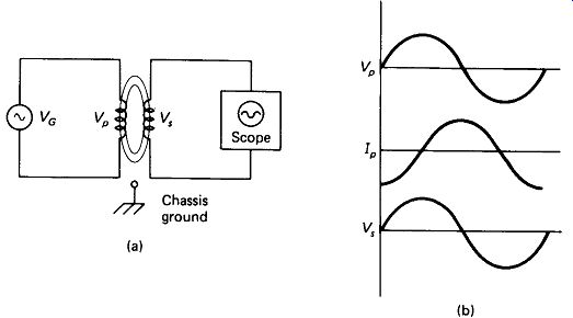
FIGURE 5-1 Basic transformer: (a) the primary creates a changing magnetic
field which induces a voltage in the secondary; (b) the secondary voltage
Is proportional to the rate of change of primary current, placing It In phase
with the input sine wave.
Isolation: You may ask: "What good is reproducing the same voltage?" The answer is: isolation. Notice in Fig. 5-1(a) that the secondary circuit is not actually connected to the primary circuit or to chassis ground. The entire Vc source may be held 1000 V above ground by another supply, but the secondary reproduction of VG can be safely tied one side to ground. This use of an isolation transformer to allow ac signals to be shifted up or down with respect to their original ground reference is quite common.
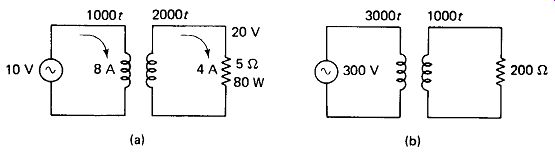
FIGURE 5-2 A transformer can step up voltage at the expense of current (a),
or step down voltage to get greater current (b), but power in must equal
power out.
Voltage Transformation: If the primary winding of an ideal transformer contains 1000 turns and the secondary contains 2000 turns, the voltage induced in the secondary will be twice the applied primary voltage. In general, where n is called the turns ratio. Now, if a load resistance is connected across the secondary, as in Fig. 5-2(a), a secondary current Is = Vs/R L will flow and a power P = IsVs WiM be delivered to the load. This power must first be delivered to the primary side of the transformer by the generator, and requires a current IP «= P/Vp, assuming an ideal transformer with no losses. Using the numbers in Fig. 5-2(a), the secondary voltage of 20 V causes 4 A through the 5-B load, resulting in 80 W of power. This requires 8 A of primary current. Thus the transformer has stepped voltage up by a factor of 2, but has stepped current down by a factor of 2. In general, for a transformer the current and voltage ratios are reciprocals:
Notice that we are using capital P and S subscripts to identify primary and secondary, respectively. We use lower case p and s to refer to parallel and series.
Of course, there must also be a magnetizing current flowing through the primary inductance, but in an ideal transformer it is assumed that this is negligible in the face of the resistive current IP which is dealt with in this formula. Remember from Fig. 4-4 that a reactive current that is one-third or less of a resistive current is negligible because of phasor addition properties.
EXAMPLE 5-1
Find the primary current in the circuit of Fig. 5-2(b).
Solution
[...]
Reflected Resistance: If the inductive primary current is neglected, the source in Example 5-1 appears to be driving a resistance R_ref = VP/IP - 300/0.167 - 1800 ohm.
This is exactly 32 (or 9) times RL. In general, the apparent or reflected resistance at the primary is
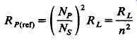
(5-3)
We say that the impedance ratio varies as the square of the turns ratio.
Looking at it from the other side, the load seems to be driven through a resistance which is the actual generator resistance multiplied by the square of the turns ratio:
s(ref) - RGn2 (5-3a)
FIGURE 5-3 Resistance is reflected across a transformer by the square of the turns ratio: (a) original circuit; (b) load resistance referenced to primary; (c) source voltage and resistance referenced to secondary.
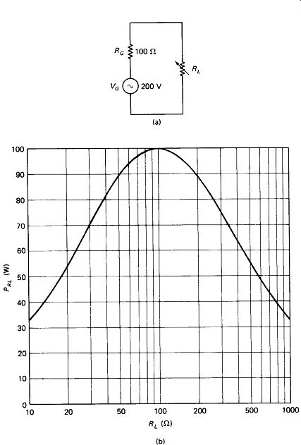
FIGURE 5-4
The reflected generator voltage is multiplied by the turns ratio n only.
Figure 5-3 illustrates the reflected resistance as seen from the primary and secondary sides
Impedance Matching: Signal sources invariably have some source resistance Rc through which they must push current to a load. This is illustrated in Fig. 5-4(a). If the load resistance is made very low, the load current will be maximized, but the power in the load will be low because the voltage across it will be low and P - IV.
If the load resistance is made high, the voltage across it will be maximized but the current will be low, again resulting in low power in the load. For any fixed Rc, the greatest power is delivered to the load when RL = Rc. We then say that the source and load impedances are matched. Figure 5-4(b) graphs the effects of matching and mismatching.
Transformers are often used to deliver maximum power to a load when the available generator resistance differs markedly from the available load resistance.
The following example will illustrate the method.
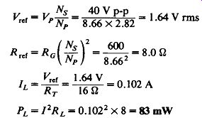
EXAMPLE 5-2
An experimenter wishes to dive an 8-ohm speaker with a 600-i signal generator in connection with an audio test. The maximum open-circuit output is 40 V p-p.
Determine the power delivered with a direct connection, and then find the transformer ratio for maximum power transfer and calculate the new power delivered.
Solution Without the transformer, as in Fig. 5-5(a):
With the transformer, as in Fig. 5-5(b), an impedance ratio of 600:8 must be matched:
-------
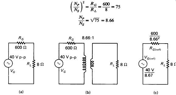
FIGURE 5-5 Impedance matching to maximize power to a load: (a) mismatched
circuit; (b) transformer provides matching; (c) equivalent circuit referenced
to secondary.
The transformer should have an 8.66-to-l step-down ratio. Note from Fig. 5-4(b), however, that this is not an especially critical number. Impedance ratio differences by a factor of 2 up or down (turns-ratio differences by V2 or 1.41 up or down) will cause only an 11% loss of load power. Assuming an ideal transformer with an 8.
66:1 primary-to-secondary turns ratio, the equivalent circuit referenced to the load appears in Fig. 5-5(c).
---------
The output power is increased 84/4.3 = 19.5 times by the transformer impedance match.
5.2 REAL TRANSFORMERS
A complete equivalent circuit for a real transformer and a photograph of some representative transformer types appear in Fig. 5-6. Fortunately, we do not have to deal with all the components shown in any single application of any single transformer. The next four sections are devoted to sorting out which parts are essential and which can be neglected, case by case.
XPk and Xsk are the magnetically coupled parts of the primary and secondary inductive reactances at the operating frequency. These parts of the real transformer behave just like the ideal transformers of Figs. 5-1 to 5-3. and X_pl are the remaining parts of the primary and secondary reactances, termed leakage reactances. Leakage reactance results from the inability to wind the primary and secondary coils perfectly close together, or from the specific intention to keep them from being too close. Thus not absolutely all of the magnetic field produced by the primary is intercepted by the secondary. We say that the coefficient of coupling k is less than unity. The actual value is given as k - XPk/(XPk + XPL). If leakage reactance becomes larger than the reflected load impedance across Xpk, the input voltage VP will be prevented from reaching coupling reactance Xpk RP and Rs are the winding resistances of the primary and secondary, respectively, and may be governed by skin effect if the wire size is large or the frequency is high. RH represents losses due to hysteresis and induced currents in the core material.
CP and Cs represent the effective stray capacitance across the primary and secondary windings, while CPS represents the stray capacitive coupling between the two windings.
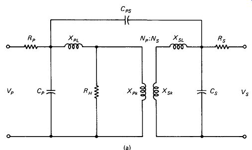
FIGURE 5-6 (a) Real transformer equivalent circuit.

FIGURE 5-6 (b) Some representative types of transformers: potted, bell-end,
and open-frame power transformers (rear), 2-W power and 0. 5-W audio transformers
(center left,), miniature audio (foreground left,), two pulse transformers
(foreground center ), and three 455-kHz parallel-tuned trans formers, one
with the shield removed ( foreground right).
5.3 POWER TRANSFORMERS
The following characteristics are assumed for power transformers in this discussion:
. Operation at a relatively low fixed frequency (50 or 60 Hz for land-based, 400 Hz for airborne equipment). CP, Cs, and Cps in Fig. 5-6(a) are therefore negligible.
. Coefficient of coupling k equals unity, so XpL and XSL are negligible.
(Typical k values for power transformers actually center around 99.8%.)
. Core losses small enough that RH is negligible, except for determining the primary current with no secondary load.
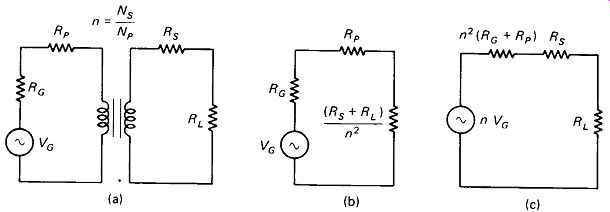
FIGURE 5-7 (a) Power transformer equivalent circuit, (b) Referenced to primary.
(c) Referenced to secondary.
The resulting power transformer equivalent circuit is given in Fig. 5-7(a). The equivalents with reflected resistances referenced to the primary and secondary are shown in Fig. 5-7(b) and (c), respectively.
Skin Effect: The skin depth for copper at 60 Hz was calculated in Example 1-4 as 0.85 cm (0.33 in.). If the wire radius is three or four times smaller than this, the skin effect can be neglected and the dc winding resistance can be used in calculation.
This is the case for all 60-Hz power transformers that are likely to appear in electronic equipment.
Power-Transformer Ratings: Unfortunately, manufacturers, specifications for electronic transformers generally include only the rms secondary voltage at the maximum rated secondary current with the specified line voltage at the primary.
This leaves numerous questions unanswered. The most useful pieces of data for power transformers are the true turns ratio and the primary and secondary winding resistances. The true turns ratio of a power transformer can be determined by simply measuring the ratio of primary to secondary voltages with no load connected to the secondary. The primary and secondary winding resistances can be measured with a dc ohmmeter unless the transformer is a real brute, in which case skin-effect resistance will have to be determined.
The IEEE has established norms for power-transformer voltage regulation eta which, to the extent that they are followed, permit an approximate calculation of true turns ratio n and Thevenin resistance from the manufacturer’s specifications of primary voltage VP, full-load secondary voltage VQ, and secondary current I0. The formulas for making the conversions are:
(5-4)
The recommended values of eta, which expresses rise in output voltage from full load to no load, are given below.
----
For example, a transformer rated as 117-V primary, 48-V, 2-A secondary, would have a regulation rj of about 6%. The true turns ratio and Thevenin resistance would be approximately ...
------
Output-Voltage Calculation: The output voltage for a power transformer supplying sinusoidal current to a load can be predicted by reflecting the primary winding resistance to the secondary side and analyzing a simple series circuit.
FIGURE 5-8 (a) Transformer and parameters for Example 5-3. (b) Equivalent
circuit referenced to secondary.
EXAMPLE 5-3
A power transformer rated at 35 V, 1 A is tested, with the results appearing in Fig. 5-8(a).
Predict the actual output voltage while supplying 1 A to a resistive load,
and determine the power loss in the transformer.
Solution The actual turns ratio is:
The line voltage and primary resistance reflected to the secondary are Kct
The equivalent circuit is shown in Fig. 5-8(b), and is easily analyzed by Ohm’s law:
The output voltage at any other load current can be predicted in a similar manner. Large overcurrents can be drawn for brief periods with no ill effects other than the great drop in output voltage. (Excessive load currents do not cause core saturation-this is explained in a subsequent section.) Of course, the power burned in the transformer goes up as the square of load current, and the heat-dissipation rule of thumb (20 mW/cm^2 of surface area for 20° C rise) presented in Section 3.5 should be kept in mind. Also keep in mind that, for large power transformers, the resistance of the ac line feeding the transformer may be significant. The exact value depends entirely upon the type of service available, but ranges typically from 0.1 to 1 B. This value should be added to the primary resistance in the analysis.
Pulsed Load Currents: The most common use of a power transformer in electronic equipment is to drive a rectifier, which in turn feeds a filter capacitor, as in Fig. 5-9(a). The current from the transformer secondary is not sinusoidal but flows in large brief pulses at the peak of the sine wave, as shown in Fig. 5-9(b). There are two important consequences of this current waveshape:
1. The voltage drop across the transformer winding resistances must be calculated using the peak secondary charging current, not merely the dc load current.
2. The power dissipated in the transformer winding resistances is, of course, I^2Rw, but I is the true rms value of the charging current peaks, not merely the dc load current.
To illustrate these points, consider that the hypothetical rectangular charging pulses of Fig. 5-9(c) apply to the circuit of Fig. 5-9(a). The total effective winding resistance of the transformer is the primary resistance reflected down by n2 , plus the secondary resistance:
FIGURE 5-9 (a) Standard rectifier circuit with capacitor filter, (b) Secondary
current (lower trace) is not a sine wave, but rather consists of brief pulses,
(c) Hypothetical rectangular charging pulses (see the text).
The average current in the secondary is 4 A X 10 ms/40 ms = 1 A, which is the load current. However, the voltage drop across Rw is due to the peak charging current, and this results in a lower peak voltage to the filter capacitor:
The average power burned in the winding resistance is calculated by the following steps:
1. Square. Find the power during the 10-ms charging period by P = I1 R:
hg = =4JXl=16W
2. Mean. Find the average (mean) power during the total 40-ms period:
10 ms av = chg x duty cycle = 16 X = 4 W
3. Root. The power-burning equivalent current can now be calculated by
The application of this root of the mean of the square technique for finding the power-burning dc equivalent of a current or voltage is relatively simple for rectangular pulses, but for most waveforms it requires calculus or computer-assisted analysis. For sine waves, the familiar results 1 ms = 0.7077pk and 7 // = 1.11 are obtained. In general, the more narrow and high-peaked the waveform, the higher the ratio / rms//av. Figure 5-10(a) and (b) gives the ratios of peak and rms currents, respectively, to average current in full-and half-wave rectifier circuits with capacitor-input filters. It is assumed that C is large enough so that it discharges to not less than 75% of its peak voltage between charging pulses. Notice that full-wave rectifiers and higher values of Rw result in lower transformer current requirements for a given RL.
EXAMPLE 5-4
Calculate the dc voltage at the load and the power dissipated in the winding resistance for the circuit of Fig. 5-9(a).
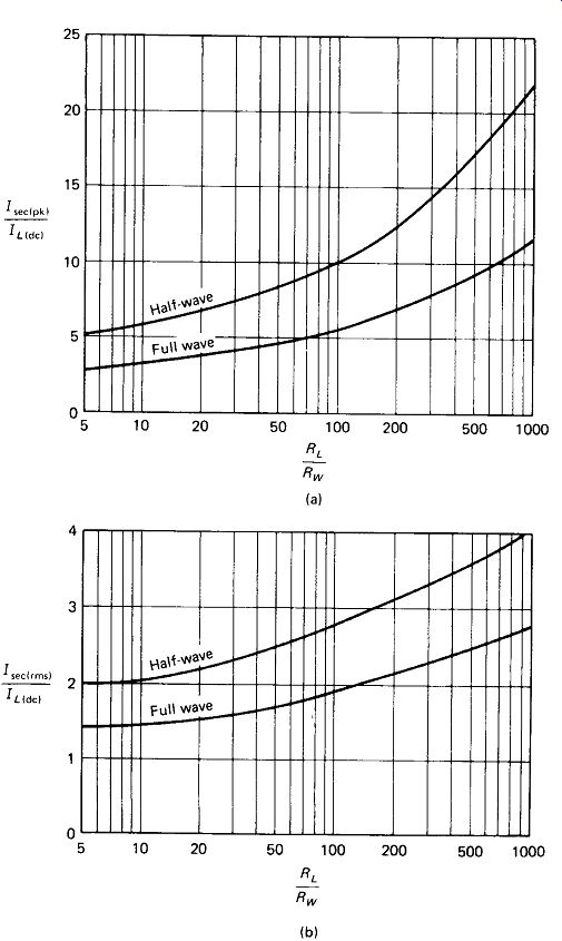
FIGURE 5-10 (a) Peak secondary current can be 2 to 20 times dc load current
for a capacitor-input filter, (b) The transformer secondary must be rated
for the true rms value of charging current, which may be from 1.5 to 4 times
the dc load current.
Solution
The effective winding resistance Rw has already been found to be 1 12. An estimate of Vout is needed to calculate RL and hence RL/RW. We will estimate K_out = 20
From Fig. 5- 10(a), the peak charging current will be 6.6IL or 6.6 A. The voltage drop across Rw is therefore that due to 6.6 A through 1 0. The load voltage is the peak reflected voltage minus the drop across Rw, minus the diode drop, which we estimate as 1.0 V:
= 20 X 1.
41 - 6.6 A x 1 ohm - 1.0 V-20.6 V
For the sake of completeness we will calculate the minimum (valley) voltage of the rippled dc, using the constant-ratio-of-discharge formula CV = It:
= 19.5 V
From Fig. 5-10(b), the rms secondary current (which must not exceed the trans former rating) is 2.1 times IL, or 2.1 A. The power in the winding resistance is Pfv= I2Rw= 2.12 X 1 - 4.4 W
The utilization of the secondary winding must be considered when applying this analysis technique to other rectifier circuits. Secondary ratings for the half-wave and the full-wave bridge circuits can be obtained directly as above. A full-wave center-tapped transformer rated at 1 A can be thought of as two 1-A windings, equivalent to a single 2-A winding, since each half-winding is used only half the time. Both the full- and half-wave voltage-doubling circuits can be viewed as two half-wave circuits, each feeding 0.5RL, so the rms current for one half-wave circuit feeding 0.5RL from actual Rw must be found and then doubled to find the secondary rating required. A choke-input filter allows nearly constant charging current if the choke is large, eliminating the peaks of charging current which produce high rms currents. Figure 5-11 summarizes the various rectifier circuits and the common ratios of:
The low ratios given are for RL/Rw= 10 and the high numbers are for RL/Rw= 100.
The ratio of 1000 is not considered because it is likely to occur only with high RL when currents are relatively low anyway.
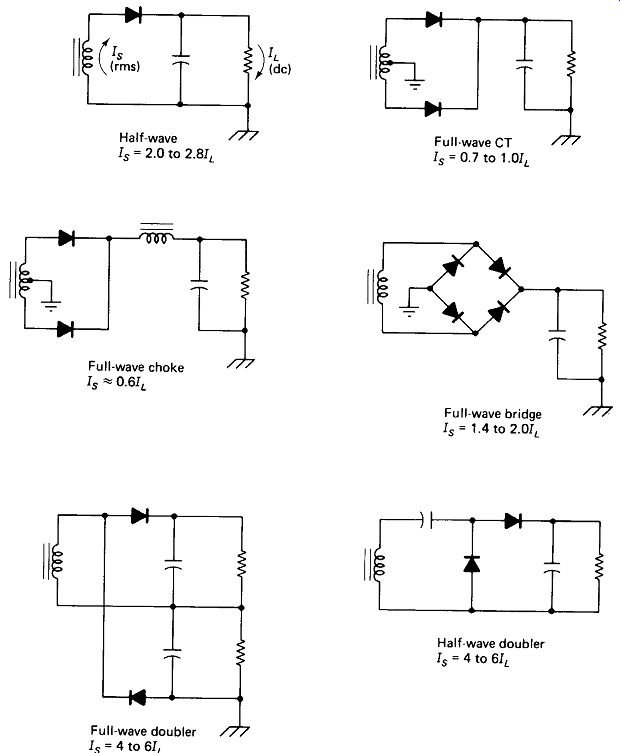
FIGURE 5-11 Recommended secondary rms current ratings for various rectifier
circuits.
No-load Currents: Although they have no effect on the ability of a transformer to supply current to a load, it may be well to consider the magnetization currents that flow in the primary of a power transformer regardless of load. Figure 5-12 shows the equivalent-circuit components involved, and the accompanying phasor diagram gives an idea of the relative magnitudes of their currents. Transformers for 60-Hz electronics equipment generally have primary inductances ranging from about 1 H for 500-W units, up to 10 H for 2-W units. The smaller transformers require higher inductance to limit the magnetizing current to avoid saturating the tiny core. The Q of the primary inductance is generally between 1.5 and 3. Most of the resistive component of primary impedance is due to losses in the core material, represented as shunt resistance RH. Series winding resistance RP is very much smaller than RH, except in the smallest transformers, where the fine primary winding may have a resistance as much as is calculated as QXP, where Q is measured on an impedance bridge, calculated from tangent of the angle between no-load current and voltage, or simply estimated as 2 for standard power transformers.
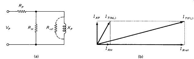
FIGURE 5-12 (a) Transformer primary equivalent circuit showing winding resistance
Rp and core-loss resistance RH- (b) Phasor diagram showing relation between
no-load and full-load primary currents.
EXAMPLE 5-5
A nominal 24-V 2-A 60-Hz power transformer has the following parameters:
Vp= 120 V Rp = 12 ohm LP= 3H Rs= 1.5SI QP = 2.5 n = 0.278
Find the power dissipated within the transformer at full load.
Solution
The core loss is computed first, using XLP and QP to find RH:
XLP = 2 pi rfL = 2 pi r X 60 X 3 = 1130 ohm
RH = QpXP= 2.5 X 1130 = 2825 0 Vp 120Z p = -L = = 5 l w e0r RP 2825
Next, the winding loss is found by reflecting RP to the secondary:
= 14.8 W
Core Saturation: The current in the magnetizing inductance XP increases with higher primary voltages or lower line frequencies. The transformer's number of primary turns and core structure have been designed for a particular voltage and frequency, and higher voltages or lower frequencies are likely to cause core saturation (see Fig. 4-16).
Load current does not contribute to core saturation because the primary current flowing into the reflected load resistance produces a magnetomotive force which exactly cancels that of the secondary load current, as illustrated in Fig. 5-13(a).
You may ask why higher-power transformers always have larger iron cores if load current does not cause saturation. The answer is that high load currents require heavier wire to minimize copper losses. This means that a larger winding form is required and that fewer turns can be fit on the form, so is lower and magnetizing current is higher for larger transformers. Transformers for 400 Hz can achieve high %LP with 2.5 times fewer turns, and do in fact use about 2.5 times less iron than that used by 60-Hz transformers. Power transformers for dc inverter-type supplies operate in the kilohertz range and are much smaller still.
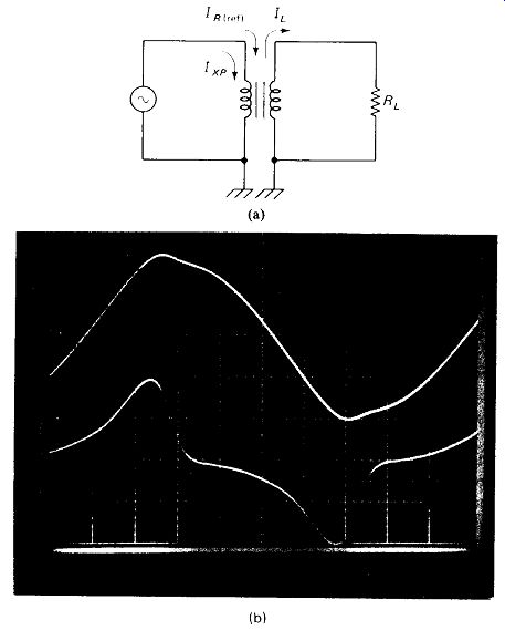
FIGURE 5-13 (a) Load current does not cause core saturation because IR(ref)
cancels its magnetizing effect, (b) Primary (upper trace) and secondary voltages
for a transformer in saturation.
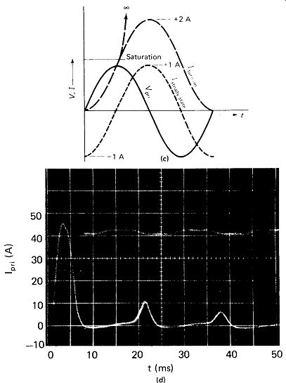
FIGURE 5-13 (c) Turn-on current starts from zero and exceeds the saturation
level if the primary is switched on at the start of a voltage half-cycle,
(d) Actual turn-on surge for a 200-W transformer with steady-state current
(inset) for comparison.
Since the ratio of voltage to frequency at the threshold of saturation is constant for any given transformer winding, a signal generator and oscilloscope can be used to check the saturation limit. Set the generator to a low frequency, say 6 Hz, and connect it to the primary. Observe the secondary waveform on the oscilloscope, watching for signs of saturation as the primary voltage is increased.
What you see at 15 V at 6 Hz is what you can expect at 150 V at 60 Hz, or at 125 V at 50 Hz. The low-frequency test is a little less destructive, however. Figure 5-13(b) shows primary and secondary voltages for an extreme case of saturation. The primary is being fed from a 50-ohm source. Notice that, when saturation is entered, the primary voltage is loaded down from its usual sine shape, and the secondary voltage simply disappears. The primary current at this time is limited only by the dc resistance in the primary circuit, and at 120 V it would be destructively high.
Core saturation often causes a tremendous current surge when a power transformer is switched across the ac line. Figure 5-13(c) shows why. At steady state (dotted line) the inductive current lags the voltage by 90° , rising from - 1 A to +1 A during the positive voltage half-cycle in Fig. 5-13(c). However, if the switch happens to close at the start of a voltage half-cycle, the current rises from an initial value of zero to +2 A provided that the core doesn’t saturate first (dashed line.) In fact, manufacturers almost never put in the extra iron and copper to prevent turn-on saturation, so primary current is limited only by primary winding resistance in the last part of the first half-cycle. Figure 5-13(d) shows the turn-on surge for a 200-W transformer reaching 45 A, while the inset trace shows a steady-state peak less than 1A.
Turn-on surge may cause trouble with fast circuit breakers or line noise.
The simplest way to alleviate the problem is to leave the primary connected permanently to the line and switch the secondary.
5.4 BROADBAND TRANSFORMERS
The following characteristics are assumed for broadband transformers in this discussion:
. Operation over a frequency range spanning at least one decade, possibly as much as five decades
. Magnetic core with coefficient of coupling of 0.75 or greater.
The chief representative of this class is the audio transformer, wound on a core of laminated silicon-iron strips. The more recent development of high-frequency ferrite materials has made possible the construction of broadband video and radio-frequency transformers, even into the UHF range.
All of the components shown in the equivalent circuit of Fig. 5-6 may become involved in the analysis of broadband transformers, with the additional considerations of skin-effect resistance, series resonance of the windings, and saturation and high-frequency loss in the core. We can keep the analysis reasonably simple, however, by concentrating on two main questions: low-frequency cutoff and high-frequency cutoff.
Low-Frequency Cutoff: A transformer can cease to function at low frequencies for one of two reasons: core saturation or inductive loading.
Core saturation can be calculated from equation 4-27 if the number of primary turns is known and the core area can be determined. It must be remembered that core saturation for any given transformer depends upon primary voltage and frequency only, as illustrated in Fig. 5-13. The result of low-frequency core saturation is not simply reduction in output, but rather waveform distortion. The cure can be a larger transformer (higher XLP or bigger A ), lower primary voltage, or limiting the low-frequency response before the signal gets to the transformer.
Inductive Loading: As signal frequency is lowered, the inductive reactance of the primary drops. At some frequency %LP will equal the Thevenin equivalent source resistance through which it is driven, and the voltage across it will then drop to 0.707 of maximum. This is illustrated in Fig. 5-14. Combining the expressions for XF, Rret, and R lh yields a formula for low-frequency cutoff:
(Rg + RA RL/n1
... where n = Ns/NP,f\s in hertz, L is in henrys, and all Rf s are in ohms.
Examination of this equation reveals that raising LP is the most effective way of obtaining the lowest possible operating frequency. Lowering Rc and Rp, and to a lesser extent raising RL, will also help.
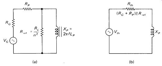
FIGURE 5-14 Low-frequency cutoff occurs when primary reactance drops lower
than effective driving resistance: (a) equivalent primary circuit; (b) Thevenin
equivalent.
High-Frequency Cutoff: The response of a transformer at high frequencies can be limited by any of three factors: leakage reactance, core losses, and series resonance.
Leakage Reactance: The coefficient of coupling of broadband transformers ranges from above 99.5% for audio types down to 80% or so for some of the low-pi ferrite toroids. In any case, the leakage reactance in the primary PL is not zero, and it appears in series between the source and the load, as shown in Fig. 5-15. As frequency increases, XPL will increase until it becomes large enough to limit the voltage across Rref to 0.707 of its midband value. In most cases, core loss R H and coupled reactance XPk are negligible compared with the low value of R„f, so the simple circuit of Fig. 5-15(b) applies and (Rc + R.) Rg+Rp+ , 2 7r ( 1 - k) Lf

(5-7)
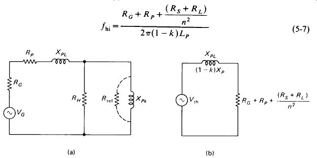
FIGURE 5-15 Leakage reactance can be great enough to cause high frequency
cutoff: (a) primary equivalent circuit; (b) Thevenin equivalent.
Notice that most of the things that will improve high-frequency response (lower LP, higher Rc, higher RP) are precisely the things that will degrade low-frequency response-such are the frustrations of life. Raising RL will aid both causes, but driving a load is usually a prerequisite, unless we can contrive to feed the secondary into an emitter follower or FET amplifier.
The real key to high-frequency response (at least this one-third of it) is a coefficient of coupling k that approaches unity, which then results in a leakage reactance approaching zero. High-A: values are obtained by keeping both coils close together on a high-k form with minimum or zero air gap. Measurement of A: is a fairly simple matter and is illustrated in Fig. 5-16(a) and (b).
A test voltage at a frequency toward the high end of the transformer midband range is applied to the first winding and the primary (F,) and secondary open-circuit (V2) voltages are measured. The transformer is then reversed, and the test voltage is applied to the second winding as the new primary, and input (K3) and open-circuit output (K4) are measured. The value of k is then found as (5-8).
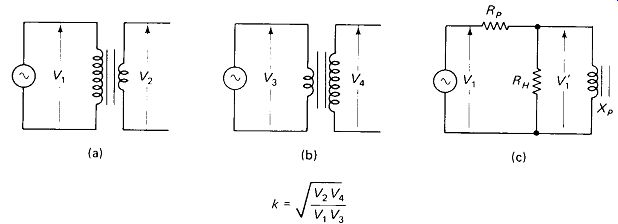
FIGURE 5-16 Measuring coefficient of coupling k is relatively simple: (a)
and (b) the basic measurements; (c) correction technique for use when k is
near unity and high precision is required.
The true turns ratio of the transformer can also be calculated from these data:
If k is within a percent or two of unity, n can be found more simply as VOM/ Vin, but as k becomes lower this calculation loses accuracy and equation 5-9 must be used.
Figure 5-16(c) shows that the Vx and V3 input voltages measured may not exactly equal the voltage across the primary reactance V’1. By making f_test relatively high, we make XP large and minimize the drop across Rp, but if it is desired to calculate k to within 0.1% it will be necessary to find the Thevenin equivalent of RP, and RH, and calculate the true value of V’1. Similar treatment must be given to V3 on the second measurement set, and of course the voltmeter used must be precise to at least 3.5 or 4 digits.
Core Losses: At higher frequencies the hysteresis losses in a magnetic material begin to increase, lowering the Q of the coil and lowering the value of RH in Fig. 5-15(a).
The methods of defense against this mode of high-frequency cutoff are:
. Use a core material with a higher maximum frequency than the application calls for (if possible).
. Use a low generator source resistance Rc.
. Use heavy primary wire to lower RP.
. Keep k as high as possible by placing the windings close together on a high-k core with no air gap.
At some frequency, generally considerably above the frequency where hysteresis loss becomes severe, the permeability of the core material will begin to drop.
Above this frequency the magnetic coupling between the windings decreases (lower k value) and no combination of circuit parameters will elicit a full response from the transformer.
Series Resonance: The most common cause of high-frequency cutoff in broadband transformers is series resonance of the primary winding. Parallel resonance of the winding with its stray capacitance presents no problem since the reactance simply increases, but when the first few turns of the primary coil resonate with the series stray capacitance from the center of the coil, a very low impedance results, which tends to load down the source. The worst part of it is that the capacitance shunts out the bulk of the primary winding, effectively increasing the turns ratio NS/NP of the transformer. An attempt to illustrate this phenomenon is made in Fig. 5-17(a).
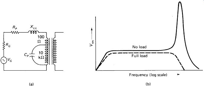
FIGURE 5-17 (a) Series resonance of the first few primary turns with the
bulk stray capacitance is the most common cause of high-frequency cutoff
in an audio transformer, (b) Dangerously high voltages can be generated at
the series-resonant frequency if the transformer is operated without a secondary
load.
With no load on the secondary, this new turns ratio will result in a severe peaking of the secondary output voltage at the series-resonant frequency, as shown in Fig. 5-17(b). The peak voltages attained can easily reach 10 times their normal values. Large signals containing high-frequency components should never be applied to an unloaded transformer, or insulation breakdown could result. The peaking problem can be completely eliminated by making sure that the secondary reflects back even a moderate load to the primary. The Q of the primary inductance and consequently the series-resonant voltage rise will thereby be reduced.
Increasing the upper-frequency limit imposed by series resonance is another matter, however. The best solution is to limit stray capacitance by keeping the number of turns low. This can be done without lowering Lp and thus ruining low-frequency response if a low-reluctance gapless core of high-μ material is used.
Spaced and cross-diagonal winding techniques for reducing capacitance are difficult to implement physically and the gains to be realized in this way are small.
Calculating the series-resonant point is chancy at best, but an estimate can be given as 3 to 10 times the parallel-resonant frequency, which can be calculated from the inductance and the estimated stray capacitance of 0.05 pF/turn.
EXAMPLE 5-6
A 50-turn to 50-turn transformer is wound of No. 22 enameled wire on a 3B7 toroid core with average diameter 2 cm and cross-sectional area 0.25 cm^2.
VG =
20 V rms, Ra = 50 12, and RL = 50 U.
Coupling k is measured as 98% per Fig. 5-16.
Predict the upper and lower cutoff frequencies.
Solution
Consulting Fig. 4-15 for u and using equation 4-25, we obtain
LP = 0.012 4 = 0Q13 X 5°2 x 2000 x = 2400 uH I LIT
The low cutoff due to inductive loading, by equation 5-6, is
Since n = 1 and Rp is negligible, this becomes
f 50 50 h° 217X0.0024 50 + 50 ,/' ktZ
Of the 20-V source, 10 V is dropped across RG and 10 V appears across R_ref. The low cutoff due to core saturation, by equation 4-27, is
= 4.5 kHz
Thus core saturation governs at the 10-V level, but/lo could be as low as 1.7 kHz if VG were limited.
High-frequency cutoff due to leakage reactance, by equation 5-7, is:
This is about equal to the limit imposed by the core material (Fig. 4-15).
A wild guess at the series-resonant point may be ventured:
= 2 MHz
The series-resonant point is therefore likely to be above 6 MHz, which is safely above the previously calculated 330 kHz.
A final calculation of the skin-effect resistance of the coil will be made to ensure that it is negligible in the face of Ra and R L. The thickness of AWG 22 wire is 0.064 cm. The total length, assuming that the core is 0.5 cm on a side, is 2 cm/turn X 50 turns, or 100 cm. Using equation 1-4 yields ... R = 0.075 ohm
Audio-Transformer Specifications: Audio-transformer ratings generally include:
. Primary and secondary impedances. These are the load resistance and source resistance with which the transformer is designed to operate over its specified frequency range, and do not directly designate the inductance or impedance of the windings themselves. The true turns ratio n can be calculated as V Zs/Zp .
. Audio-power rating. This limit is generally imposed by core saturation at the low-frequency limit, and can be increased considerably if the audio lows are attenuated before reaching the transformer.
. Winding dc resistances. These are often high enough to enter into dc bias calculations. They also impose a power limit on the transformer due to the I^2R loss in each winding, and the resultant temperature rise.
. Maximum dc winding current. Transformers frequently carry dc as well as ac, and the dc contributes its own I^2R heating. If the winding is single-ended, dc also contributes toward reaching the saturation limit. In " push-pull "center-tapped transformers the dc flows into the center and equally out each end, so the magnetizing effects cancel.
. Frequency response. This is given for the primary and secondary impedances (resistive Rc and RL) specified. If Rc and Rt are lower than specified, a downward shift in the response range may be expected. Raising Rc and RL will raise the lower cutoff but probably not the upper cutoff, since it is most likely to be due to series resonance of the winding.
The Audio Range: Considerable research has gone into determining the range of frequency response required for audio reproduction, with the following fairly well- accepted results:
Range (Hz) | Application
300-3500 Understandable voice communication
80-8000 Natural voice, reasonable music
50- 15,000 Good-fidelity music
15-20,000 Extremely high fidelity
Analysis of typical audio waveforms shows that they tend to have higher peaks with lower effective (rms) values than do simple sine waves.
This means that saturation and other peak-clipping phenomena are likely to be more troublesome than power-dissipation limitations in audio systems. A two-tone test-two signals added, for example, 400 Hz in series with 1 kHz-is often used to simulate an audio waveform.
5.5 RADIO-FREQUENCY TRANSFORMERS
In dealing with RF transformers we can expect to encounter a rather wide range of physical device forms and a variety of design objectives. Among the devices:
. Ferrite toroid core transformers; k values from 0.80 to 0.98; generally unsuitable at high power levels because of core saturation
. Powdered iron slug-tuned transformers; k values around 0.75; also susceptible to saturation at high levels
. Air core transformers; no saturation or nonlinearity problems; k values depending on structure:
bifilar winding (two strands wound together side by side) k - 0.95 primary over secondary (single layers, 1:1 ratio) k - 0.90 link coupling (2 or 3 turns over 10 or more turns) k ~ 0.60 end-to-end coils (length = diameter) k - 0.35 end-to-end coils (length = 2 diameters) A: -- 0.10 in-line separated by one length (length = 2 diameters) k - 0.02 Among the objectivities:
. Transfer power from a source to a load, possibly with impedance step up or step down
. Tune (select) a band of frequencies while rejecting others In general, the more we try to transfer power, the less sharply we will be able to tune; and the more sharply we wish to tune, the less will we be able to transfer power.
Untuned RF Transformer: For an untuned rf transformer to be successful, the coefficient of coupling must be high (say, above 60%), so it is necessary to use toroid cores at low power levels and winding-over-winding air-core structures at high power levels. Figure 5-18 shows the transformer equivalent circuit, and simplifications referenced to the primary and secondary, respectively. The latter is most useful for analysis of results at the load. The " prime " marks indicate reflected values; voltages are scaled by n and impedances by n 2.
If n = 1, the original values apply, of course.
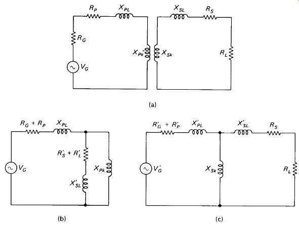
FIGURE 5-18 Untuned RF transformer: (a) basic equivalent circuit: (b) referenced
to primary; (c) referenced to secondary. Leakage reactance is usually the
factor that limits output.
Examination of Fig. 5-18(c) will show that maximum power is delivered to the load when the primary and secondary leakage reactances are kept small in comparison to the generator and load resistances, respectively, and when the corresponding coupled reactances are kept large in comparison to Rc and RL. A high-& value achieves both of these conditions at once, so winding a coil with the closest possible coupling is of prime importance. Beyond this, a decision on the number of turns required for each coil must be made. Much calculation with Fig. 5-18 can be done to find the optimum coil reactances, but it turns out that if we choose Xf = Rg and XS = RL, very little improvement in power transfer can be made, and this simple rule of thumb is recommended where k is below 90%. For higher k values, XP = 2 Rc and Xs = 2RL will give noticeably greater output.
Above the design frequency, XPL and SL will become large enough to block current to RL. Below the design frequency Xpk (or XSk, depending on how you look at it) will become small enough to shunt the output, causing all the voltage to drop across Rc. If k is large (0.90 or so), there will be quite a bit of room between these two cutoff points, and bandwidths spanning more than one decade may be achieved easily. Low-A: values will result in narrower bandwidths, however.
EXAMPLE 5-7
An untuned rf transformer consists of a 40-turn primary wound over an 80-turn secondary, both of AWG 32, both spaced over 2 cm on a 1-cm-diameter form.
Measured k is 0.80. Ra = 75 12 and RL = 300 U. Kc(open circuit) is 2.5 V rms. Find VRL at the optimum frequency /.
Solution First the inductance of the primary and the frequency where XP = RG are found:
d1Ni 402 L" = 46f+T0l7 = 46 + 202 " 6 45 "t <4"19>
2ttL = 2tt X 6.45 jiH " 1 85 MtZ
The inductive reactances, coupled and leakage, are found next. Xs is related to XP by:
Then skin-effect winding resistances are found:
Considering the proximity effect, the primary resistance is estimated as ten times the calculated value or 7 Q. Secondary resistance is 14 ohm. Figure 5-19(a) shows the circuit with the values calculated above. The equivalent circuit with primary values referenced to secondary (marked with a prime) is given in Fig. 5-19(b). The method of solution for Krl will be to obtain the parallel equivalent of %SL and Rs + RL, combine the resulting parallel XL with XSk* and convert back to a series equivalent, shown in Fig. 5-19(c).
Solution for ZT and Vab is straightforward in this circuit, and knowledge of VAB in Fig. 5- 19(b) leads directly to 1L and vRL. The parallel ...

FIGURE 5-19 Example 5-7; analysis of an untuned FtF transformer circuit:
(a) equivalent circuit; (b) referenced to secondary; (c) simplified to a
simple series circuit.
... equivalent of 60 0 inductive and 314 0 resistive in series:
(4-10)
AS X IIA' 1703 X 240 21 n f2 Xp\\Xsk 1703 + 240 210 Si
The series equivalent of 210 inductive and 325 11 resistive in parallel:
Now, looking at Fig. 5-19(c), we obtain
Zr= Vx1 + R2 = V2082 + 4242 =472 Q ft= = 14 = 0 °1°f A Zr 472 VAB = = 0.0106 Vl48Z + 96Z = 1.87 V
Returning to Fig. 5-19(b), we find that
= 0.
00585 A V602 + 3142 VRL - IlRl = 0.00585 x 300 = 1.75 V
Anyone willing to repeat these calculations for a few other frequencies will find the following results:
Series-Tuned RF Transformer: When coefficient of coupling is low and Rc is less than XPL, it will be advantageous to cancel the primary leakage reactance with a series capacitance. Cancellation will occur only for a narrow band of frequencies, so the broadband characteristic of the transformer will be lost if this technique is employed.
On the secondary side, a series-tuning capacitor to cancel leakage reactance XLS will also increase output, but again, R L must be lower than X ls if the increase is to be significant.
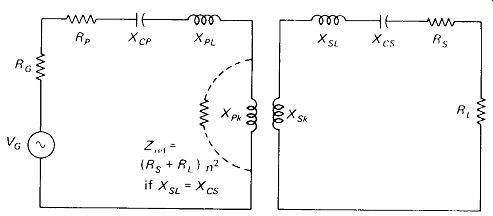
Fig. 5-20
With both the primary and secondary series tuned, much lower coefficients of coupling can be tolerated with good power transfer than in the untuned transformer.
However, very low values of k produce very low coupling reactances XPk, and this tends to short the source. Attempts to raise the input impedance by increasing the primary inductance may be helpful to an extent, but will require more windings and result in larger losses in winding resistances RP and Rs. The best approach with series-tuned transformers is to keep k at least reasonably high (say, 0.10 minimum).
The required values of the primary and secondary tuning capacitors are interactive because of the reflected impedances that appear across the coupled reactances. With reference to Fig. 5-20, let us assume that Xcs impedance reflected across Xpk is purely resistive; Rref = (Rs +RL)/n2 to be exact. The parallel combination of Rref and Xpk has a series equivalent (call it Rs and Xs) and it is the sum of Xs and XP[ which should be canceled by A'cp to achieve maximum current to the secondary and maximum power to the load.
Smaller values of secondary capacitance will result in a net capacitive reactance in series with the reflected RL appearing across Xpki which will raise the effective reactance and require a smaller tuning capacitance X' cp- Likewise, larger Cs will require larger CP values. All of this could be analyzed by methods similar to Example 5-7, but it is probably not worth the effort, since CP and Cs are generally variable and easily optimized.
The overall Q and hence the bandwidth of the circuit of Fig. 5-20 depends upon the ratios of reactance (Xc or XL) to resistance in the primary and secondary circuits. If k is large, Q is approximately the average of primary and secondary Q.
If k is small, the separate response curves of the primary and secondary are multiplied, resulting in an overall response curve that is narrower at the top than a single response curve, and drops more quickly to zero.
Note that if RL is higher than X_SL series secondary tuning will provide little improvement in selectivity or power output. Similarly, if Rc is higher than XPL, series primary tuning will not be necessary.
Parallel Primary Tuning: If the generator resistance is higher than the primary inductive reactance, it will be advantageous to parallel-resonate this reactance with a capacitor across the primary so that the generator sees a higher-impedance load.
This technique will be especially effective if k is low or if RL is high, because in either of these cases the primary impedance will be largely inductive, with only a small resistive component.
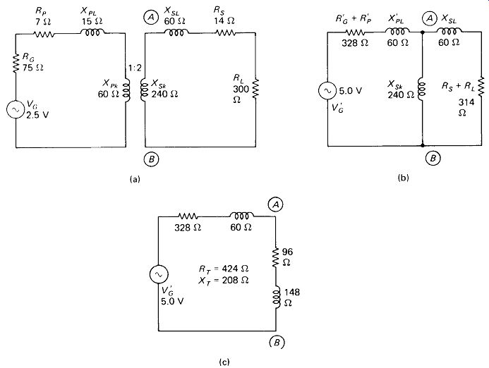
FIGURE 5-21 Parallel-primary series-secondary tuning prevents loading of
high impedance source and allows match of an 8100-ohm source to a 200-ohm
load with a 1:1 transformer: (a) equivalent circuit; (b) referenced to primary
with Rr#, and X pk converted to series equivalent; (c) simplified parallel
equivalent.
Figure 5-21 shows an example of parallel primary tuning used to effect an impedance match between an 8.1-kl source and a 200-8 load with a simple 1:1-ratio transformer having a k of 20%. The - 800-i secondary capacitance cancels the secondary leakage reactance, placing the 200-0 resistive load directly
= XSL, so that the across the secondary. The 1:1 ratio reflects this 200- ohm resistance across the 200-Q primary reactance, a parallel combination that is equivalent to 100-ohm XL and 100-12 R in series. The series branch ABC in Fig. 5-21(b) is converted to its parallel equivalent in Fig. 5-21(c). The 900-ohm primary reactance is parallel-tuned to infinity by CP, leaving only the parallel equivalent of the 100-0 Rs, which (quite fortuitously) happens to equal the source impedance of 8100 ohm. Reference to equation 4-16 will verify this.
The voltage across the primary is thus \ VG, or 5 V. The voltage across points BC is found by phasor voltage division:
This voltage is transformed undiminished to the load. Winding resistances have been neglected in this example.
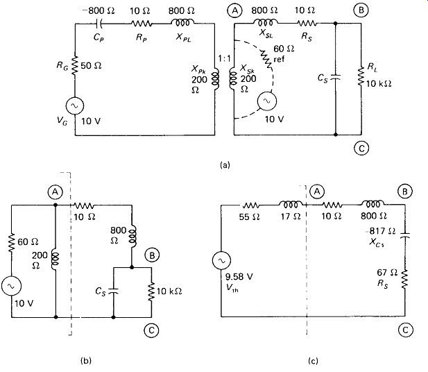
FIGURE 5-22 Series-primary parallel-secondary tuning. Secondary is actually
series-resonant, giving voltage increase across output: (a) equivalent circuit;
(b) referenced to secondary; (c) reduced to simple series equivalent.
Notice that the inductive reactance of the primary would be low enough to seriously load down the source were it not parallel-tuned by CP. We are thus able to use fewer turns in the rf transformer coils if parallel tuning is employed, and this in turn cuts down on winding-resistance loss and cost.
Parallel Secondary Tuning: If the load resistance is very high and the coefficient of coupling is low, the secondary of an rf transformer may be resonated with a parallel capacitor to achieve an impressive gain in output voltage, even with a 1:1-ratio transformer. Figure 5-22 illustrates the technique. Although the term parallel resonance is used, notice from Fig. 5-22(b) and (c) that series resonance and the accompanying voltage rise across the capacitive reactance (Section 4.3) are actually involved.
An analysis of the circuit with the values given requires finding the Thevenin equivalent of the reflected VG and 60 ohm as shunted by the 200-0 XL. Finding the = 9.
58 V series equivalent of Cs and finding the output Vbc becomes a simple matter:
(4-7)
(4-8)
Using the approximation equations 4-15 and 4-16, we let Cs cancel the total inductive reactance of Fig. 5-22(c):
The resonate voltage rise (nearly six times in this example) will be less if Rc is higher or if RL is lower. Of course, very low Rc, very high RL, and higher leakage inductance XSL can produce a circuit with a Q, and accompanying voltage rise, of 100 or more.
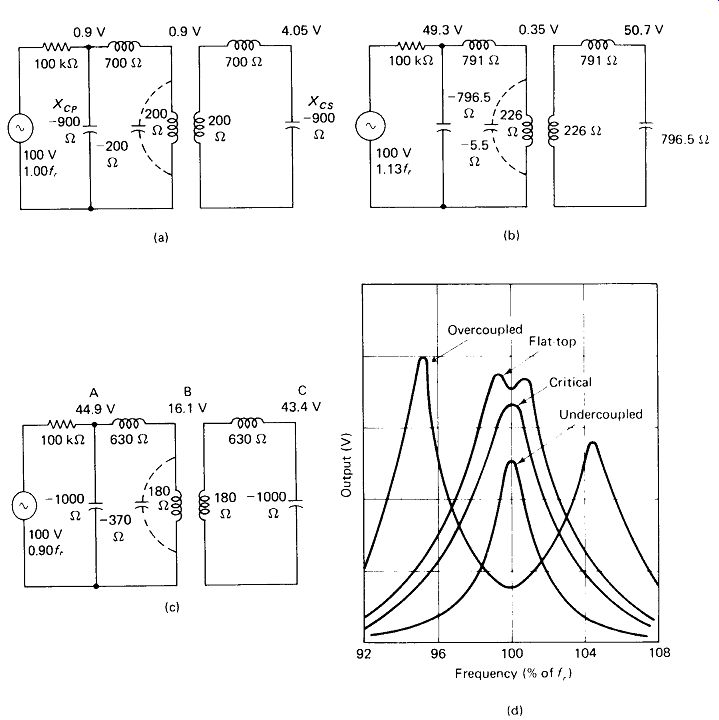
Double Parallel-Tuned Transformer: If the generator and source resistance are both very high, an effective voltage transfer can be achieved with a loose-coupled transformer parallel tuned at both the primary and the secondary. This method of tuning is widely used to achieve selectivity in radio and TV receivers.
The primary and secondary tuning are interactive because of reflected reactances across the primary, as is true in the previously discussed double-tuned circuits. However, in this case the reflected reactances can cause a double-peaking effect which is not present in the other circuits. Neither of the peaks occurs at the actual resonant frequency [Fig. 5-23(a)]. The high-frequency peak [Fig. 5-23(b)] occurs when XSL equals Xcs and a very low impedance is reflected back across XPk, leaving XPL to resonate with XCP. The low-frequency peak [Fig. 5-23(c)] occurs when the capacitive reactance reflected back across Xpk raises the total primary reactance just enough to cause parallel resonance with XCP. In practice, the low-frequency peak is always somewhat stronger because of the greater winding-resistance losses incurred with the low-impedance series-resonant condition of the high-frequency peak.
FIGURE
5-23 Analysis of a double-parallel-tuned transformer: (a) at resonance; (b)
above resonance with XSL nearly equal Xcs; (c) below resonance, with reflected
capacitive reactance causing primary re-resonance; (d) typical response curves
for the double-parallel-tuned transformer, showing effect of varying k.
The calculations for Fig. 5-23(c) are reproduced below to demonstrate the method of analysis. Calculation at a number of other frequencies (an ideal job for a programmable calculator) produces the curve of Fig. 5-23(d). Analysis of the circuit of Fig. 5-23 has been simplified by assuming that RL is infinite and Rw is zero. This results in an indeterminate division of zero by zero in the calculations at the exact peak points, so Fig. 5-23(b) and (c) show data at frequencies closely approaching the peak points.
For Fig. 5-23(c), the reactance looking out of the secondary is Xs = -1000 + 630= -370 f t This is reflected across XPk, giving the parallel result:
This inductive reactance adds to XP,:
The parallel is nearly resonant with XCP:
The voltages are, by phasor voltage division:
The effect of these reflected reactances diminishes as coupling k is reduced and Xpk becomes much smaller than XPL. The peaks become closer together and the dip between them less severe. If k is made variable, a point can be found where the two peaks merge to form a fairly flat-topped response curve with steep-sloped sides. This curve is ideal for broadband signals such as TV or FM radio. At a still lower k value, a point is reached where only a single peak exists. The exact value of this critical coupling depends upon the Q of the primary and secondary circuits:
(5-10) (5-11) (5-12)
Below critical coupling, voltage output drops off and bandwidth decreases. The Q (selectivity) of the total transformer at critical coupling is An examination of the foregoing equations will show that the highest output with sharpest tuning is obtained by making QP and Qs as high as possible, and then adjusting k for critical coupling, or slightly more if flat-topped response is desired. Highest Q is obtained with a high L/C ratio, so the coils are often resonated with only their own stray capacitance. Typical values encountered in practice are Q = 100 and k = 0.01. This can mean a physical spacing between the coils that is several times their length.
Stagger tuning (tuning the primary to a slightly different frequency from the secondary) can also be used in an under-coupled circuit to achieve a flat-topped response curve. Overcoupling is to be preferred, however, because stagger tuning results in several times less output voltage.
5.6 PULSE TRANSFORMERS
Pulse transformers are used to handle rectangular rather than sinusoidal waveforms.
Although they may provide voltage step-up or step-down, they are most often used to provide ground-reference isolation between the primary and secondary circuits.
They are generally ferrite-core devices, and must have an inductance and saturation level appropriate to the period and voltage of the pulse they are intended to carry.
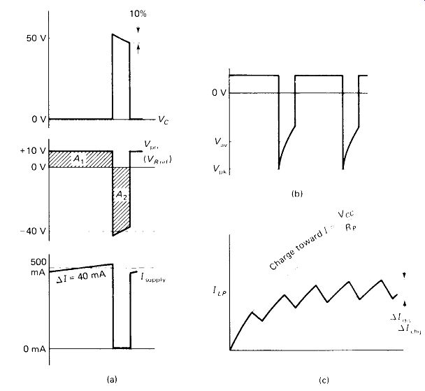
Inductance Requirement: Figure 5-24 shows a pulse-transformer circuit. Co efficient of coupling k and turns ratio n are both assumed to be unity. When the generator applies a voltage step, the current in LP will build up and the voltage across Lp will fall off according to the familiar time-constant curves of Fig. 5-24(b).
The voltage across Ls will be an exact reproduction of that across LP.
If this...
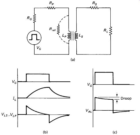
FIGURE 5-24 (a) Pulse-transformer circuit, (b) Voltage and current waveforms
in response to a pulse from VQ. (c) Droop becomes more severe if primary
inductance is insufficient.
... voltage is to maintain a reasonably square shape, the active pulse time t (when the generator voltage is nonzero) must be much less than the time constant t. If
/ = O.It, the output waveform will droop by about 9%. If t = O.Olr, the droop will be 1%. The resistance involved in this time-constant determination is the Thevenin equivalent driving LP with Rs and RL reflected to the primary. The primary inductance requirement is therefore:
LP=lOtR (for 9% droop) (5-13)
LP=lOOtR (for 1% droop) (5-14)
where
R = (Rc + RP)\\(Rs + RL)/n2 (5-15)
FIGURE S-2S Low-level pulse passes through transformer (up per trace,), but high-level pulse exceeds Vt constant and Is cut oft ( " center trace.).
Reducing pulse period allows full pulse to pass without saturating core (lower trace)
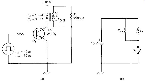
FIGURE 5-26 (a) Transistor-switched pulse-transformer circuit, (b) Equivalent
circuit with RL reflected to primary.
Volt-Microsecond Limit: Once we have assured that the primary inductance is adequate for the pulse length, we must also be sure that the primary current does not become large enough to saturate the core. Notice from Fig. 5-24(b) that primary current increases with time while secondary current decreases. The secondary current does not cancel the primary current magnetizing force for square waves as it does for sine waves. This difference between primary and secondary current increases quite linearly with time during the first portion of the time constant, and the net magnetizing force may eventually become high enough to saturate the core. If the generator voltage is increased, these two currents, and hence the difference between them, will increase, resulting in earlier saturation. For any magnetic-core transformer the maximum product of VGt before saturation is a constant:
V_G t_pulse = constant (5-16)
Figure 5-25, top trace, shows a long low-level pulse at the secondary of a pulse transformer. In the center trace the voltage has been increased, exceeding the Vt constant, and the last half of the pulse is missing. In the bottom trace the pulse period t has been reduced, bringing the Vt product back below the saturation level, and the stronger, shorter pulses are passed completely.
Transistor-Switched Pulse Transformer: The circuit of Fig. 5-26, or something like it, appears frequently enough to merit special attention, especially since its behavior is not quite as might at first be expected. In order to simplify the analysis we will make the following assumptions:
1. The transistor is a perfect switch: zero resistance when on, infinite resistance when off.
2. The transformer has unity coefficient of coupling and does not saturate.3. The transformer winding resistances are low enough to be negligible compared to RL.
4. The charging time constant LP/RP is much longer than the on time set by the pulse generator.
5. The discharge time constant LS/(RS + RL) is much longer than the off time set by the pulse generator.
None of these assumptions is unreasonable except 5 and, in some cases, 3. The effect of high winding resistance (assumption 3) is simply a reduced load voltage.
The amount of this effect can be predicted by simple voltage division. The effect of discharge occurring over an appreciable part of the time constant (assumption 5) can be estimated graphically, as will be shown later.
Using our assumptions, we draw the equivalent circuit of Fig. 5-26(b) and the graph of Fig. 5-27(a). Assumption 2 guarantees that the waveshape across Rnt (the primary) will be identical with that across RL (the secondary.) Assumptions 4 and 5 guarantee that the inductor current will rise and fall linearly.
FIGURE
5-27 (a) Waveforms for Fig. 5-26: collector voltage kicks up to 50 V during
short off interval; primary voltage must average zero, making A, - A?; collector
current shows I during on interval and I - 0 during oil interval, (b) Lower
values of Lp produce spiked kickback voltages as L discharges more quickly,
(c) Charging rate stays relatively constant at turn-on, while discharge rate
increases from zero until equilibrium is reached.
The voltage across LP and RTef is obviously cc during the on time. The fact that the average (or dc) voltage across an inductor must be zero demands that the voltage across Rre, during discharge is determined by the ratio of on to off time:
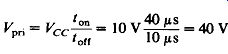
(5-17)
Graphically, this is illustrated in Fig. 5-27(a) by the equal areas Ax and A2.
Qualitatively, this means that a long on time and a short off time allows LP to build up a large current during on, which then produces a large kickback voltage during off. Quantitatively, the current change can be calculated from the charging conditions:

(5-18)
The A/disch during to[f must be the same at steady state.
The average value of ILP can be determined in the following manner:
1. Calculate the average power in Rrcl from Von and Voff.
2. Calculate the average current from the supply using Pav and Vcc.
EXAMPLE 5-8
Calculate the load voltage and supply current for the pulse-transformer circuit of Fig. 5-26(a).
Solution
The load resistance is first reflected to the primary:
The 10-ohm Rs and 0.5-ohm R_P alter this value by less than 1 % neglected (assumption 3).
The charging and discharging time constants are found:
... and are therefore …
Assumptions 4 and 5 are valid, although is only ten times t_off and some distortion of the output wave will be observed.
The voltage across Rref during /on is 10 V.
The voltage during tolf is determined by the toa/tM ratio:
This is a kickback voltage produced by the inductor current decreasing from the value it attained during toa.
Its polarity is negative at the top in Fig. 5-26(b).
The power in Rref is thus 102/100 = 1 W for the 40 /ts of /on and 40Z/100 - 16 W for the 10 ixs of /ofr.
The average power is then:
Theoretically, there are no power-dissipating elements in the circuit except R„i, so the average current from the supply must be:
In practice, we must expect /av to be 10% to 50% greater than this calculation because of transistor switching-time and saturation limitations and transformer losses. Also, the supply current is zero during to fl, so the ideal tOD supply current is:
The change of current (rise of IP during /on) is:
The load voltage VRL is simply NS/NP times VRnf, namely 50 V positive and 200 V negative. Note from Fig. 5-27(a), however, that the negative voltage peaks approximately 5% greater than its 200-V average and droops by 10% during t_off.
This is because / off occupies about 10% of r . Figure 5-27(b) shows how will greatly exceed Kav during /off if a small inductor, high RL, or long totf makes shorter than t off.
Figure 5-27(c) shows how /av is approached over several cycles after initial turn-on. A/ chg is essentially the same each ton period, but A/ , increases as ILP increases at each t off period.
5.7 STRAY TRANSFORMER EFFECTS
There are a number of instances where the transformer effect is evident , although the physical structure involved is not a transformer in the usual sense.
Stray Coupling of Chokes and Transformers: The slight amount of leakage magnetism from an iron-core choke or transformer can induce an undesired voltage in a transformer or choke that is mounted nearby. In one test at 60 Hz, 10 V across a 0.5-H choke induced 50 mV across the open terminals of a second choke mounted adjacent to it. The following techniques can be used to combat this problem.
. Keep high- and low-level inductors away from each other on the chassis. Especially watch power-supply filter chokes and audio transformers.
. Mount chokes and transformers with the axes of their windings at light angles if interference is a potential problem. This is especially effective with RF air-core coils which have high leakage reactance.
. Do not operate low-level inductors with very high load impedances unless necessary. Load current will cause stray signals to be dropped across the high leakage reactance.
. Use magnetically shielded transformers.
Current Loops in Nearby Conductors: Shield cans, metal components, or the chassis, if within range of an inductor's magnetic field, will act like loops of wire, and currents will circulate in these little " secondary windings."
The resulting I7R loss will lower the Q of the coil. Air-core coils should therefore be kept several diameters away from metal objects if highest Q is desired.
Magnetic-Field Cancellation: Iron-core transformers sometimes have a heavy copper strap bound around the laminated core. Stray magnetic fields from the transformer’s leakage inductance will induce a current in this loop, and this current will set up a field which tends to cancel the original stray field.
Variable Inductors called Variometers are made by setting up one coil which can be rotated within the other so that their magnetic fields either aid or oppose.