Why Limiters Are Necessary. The need for limiters in FM sets arises not from any intrinsic property of an FM wave but because of the limitations of some of the FM detectors currently in use. These detectors are, in varying degrees, sensitive to amplitude variations in an FM signal. As a result, the audio output contains voltages due to both the frequency modulation and the amplitude modulation. The insertion of a total or partial limiter substantially removes the AM and presents to the detector a wave that is wholly FM. Just how much limiting is required will depend upon the type of detector employed. The Foster-Seeley detector requires at least one stage and should preferably have two.
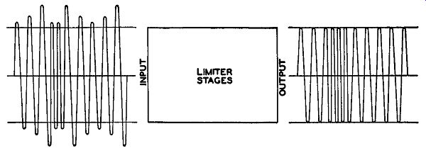
Fig. 8.1. The limiter
removes the amplitude variations (modulation) from the input signal.
The ratio detector frequently operates with out any limiters, but some limiting is desirable. The 6BN6 and 6DT6 do their own limiting. However, all FM detectors are sensitive in some degree to amplitude modulation; not one responds only to FM.
Limiter Operation. A limiter performs its function of removing amplitude modulation by providing a constant amplitude output signal for a comparatively wide variation in input voltages. A simple illustration is shown in Fig. 8.1 where the forms of the input and output voltages of a limiter are indicated. A more exact representation of the ability of a limiter to remove AM from a wave is given by the characteristic curve of Fig. 8.2. For all signals possessing more than a certain minimum input voltage at the antenna, the limiter produces a substantially constant output. In this region, starting at point B and extending to the right, the stage is purely a limiter in its action.
In the region from A to B, however, the stage functions as an amplifier because different input voltages produce different output voltages. Any signal too weak to drive the limiter beyond ( or to the right of) point B will cause amplitude variations in the discriminator output that are in no way part of the original FM signal. This represents distortion. For proper operation, it is at all times necessary that sufficient amplification be given an incoming signal in order that it arrive at the limiters strong enough to drive the tube beyond point B. Assuming that the FM signal, as it leaves the transmitter, is wholly frequency-modulated with no amplitude variations, there are two general
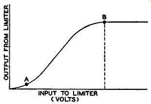
Fig. 8.2. For proper limiting action, the input voltage must be sufficiently
strong to operate the limiter at point B or beyond.
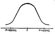
Fig. 8.3. Conventional selectivity characteristics.
points in the path of the signal where amplitude variations may be inserted. First, there are atmospheric disturbances, completely random in nature and covering every frequency used for communication. The disturbances may come from natural sources, chiefly electrical storms, or they may come from man-made devices, such as the sparking in automobile ignition systems, electrical machines, etc. Again, there are other stations that may affect the desired signal, although, for the most part, careful assignment of frequencies will minimize such interference. These are all sources external to the receiver and, largely, beyond the control of the set designer.
Within the receiver itself, the unequal response of the tuned circuits is the second important contributing factor toward amplitude variation within an FM wave. The ideal response curve is a rectangle. This, however is seldom achieved with practical equipment. Economic considerations impose restrictions on the maximum cost of the tuned circuits. As a compromise, the sloping response characteristic is employed with most tuning circuits.
An FM signal applied to a tuned circuit having the response shown in Fig. 8.3 will receive amplification dependent upon the frequency. The center frequency, to which the circuit is peaked, receives the greatest amplification.
As the signal frequency moves closer to the ends of the band, the attenuation increases.
Influence of Limiters. In order for a limiter stage to be effective, it must function beyond the knee of its characteristic curve for all frequencies of the received FM signal. In this respect the limiter has a very decided influence over the design and selectivity of the I.F. stages and the amplification that these stages must be capable of providing. Let us consider, for example, the single limiter characteristic shown in :Fig. 8.4. According to the graph, the knee of this limiter curve is reached for inputs of 15 microvolts at the antenna. As long as the incoming signal has this value, the limiter will function at saturation and no amplitude variations will be obtained at the output. Now consider the curve of Fig. 8.5. This shows the overall selectivity of a typical receiver from the antenna to the limiter. Examination indicates that the farther we move from the mid-frequency to which the receiver is tuned, the greater the attenuation to which the signal is subjected. Thus, at a point 65 khz from the carrier frequency, the signal is subjected to an attenuation rating of 1.25. Glancing back at Fig. 8.4, if 15 microvolts is required at the carrier frequency to give limiter saturation operation, then one and a quarter times this amount, or 19 microvolts, would be needed to produce the same result for that portion of the signal 65 khz off response.
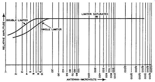
FIG. 8.4. A comparison of the input signal voltage required to produce
constant output from single and double limiters.
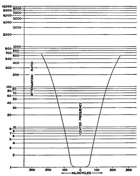
FIG. 8.5. Selectivity curve for an FM receiver tested.
Frequencies 75 khz distant are attenuated about two times the mid-frequency value and, at 100 khz, the attenuation ratio is 7. Thus, if we compute the sensitivity of a receiver at points 100 khz off resonance, we find that we need signals of 105 microvolts for complete limiting action. All this is highly important in designing the characteristics of the intervening I.F. stages and the limiter. Beyond ±100 khz, high attenuation of the signal is desirable as this minimizes adjacent station interference.
In practice, with current production limitations for the frequencies near 100 khz, the following gains can be obtained from the various stages of a well designed FM receiver.
Directional antenna ... 5x
Each R.F. stage ... 8x
Converter 15x
Each I.F. stage (except the one preceding the limiter) . 50x
I.F. stage preceding limiter 40x
Single limiter ... 2.5x
Cascaded limiters ... 6x
For complete saturation of most limiter stages, an input voltage of 2 volts is necessary. With a 10-microvolt receiver sensitivity (meaning the receiver will reproduce clearly all signals of 10 microvolts or more) an overall gain of 2 volts/10 microvolts, or 200,000, must be available for the signal prior to its application to the grid of the final limiter stage. It then depends upon the designer what combination of R.F. and I.F. stages he will use. Note the relatively poor gain of the R.F. system as compared to each I.F. amplifier.
The real usefulness of the R.F. stages lies in their partial discrimination of undesirable signals, and the boosting of weak signals to improve the signal to-noise ratio. The front end of the receiver is particularly vulnerable to extraneous voltages and anything that will help keep these to a minimum is desirable. However, as far as gain is concerned, it is far more advantageous to add I.F. stages than R.F. stages.
The lower gain obtained from the I.F. amplifier that just precedes the limiter is due to the loading effect of the limiter on the I.F. stage. Grid-current flow in the limiter (as we shall presently see) acts to lower the impedance across the I.F. output coil. The result--a decreased overall impedance with a corresponding lowering in gain. The relationship between amplifier gain and load impedance has been previously given.
Limiting Methods. There are two widely used methods for obtaining the desirable limiting action.
First, we may use grid-leak bias. This limits the plate current on the positive and negative peaks of the incoming signal. Second, we can limit by employing low screen and plate voltages, producing what is known as plate voltage limiting. Many designers combine both methods in one stage and obtain a better degree of limiting.
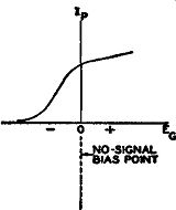
FIG. 8.6. The no-signal bias point for a limiter stage using grid-leak
bias.
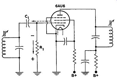
FIG. 8.7. A grid-leak bias limiter stage.
Grid-Leak Bias Limiting. The principle of operation of a grid-leak limiter is not difficult to understand. Initially there is no bias and the tube is operating at the zero bias point of its E0lp curve. This is shown in Fig. 8.6. Upon the application of a signal, the grid is driven positive and current flows in the grid circuit charging up capacitor C1 (see Fig. 8.7). It is easier for the current to charge C1 than to attempt to force its way through the relatively high resistance of R1. The capacitor continues to charge throughout the entire portion of the positive half of the incoming signal.
During the negative portion of the input cycle, the accumulated electrons on the right-hand plate of C1 flow through R1 and the coil to the left hand plate. The capacitor discharges because it represents a potential difference and, as long as a complete path is available, current must flow. The electrons passing through R1 develop a potential difference with the polarity as indicated in Fig. 8.7. From the moment the input voltage departs from its positive values to the beginning of the next cycle, the discharge of C1 continues.
At the start of the next cycle, there will be some charge remaining in C1, Hence, the grid does not draw current again until after the input voltage has risen to a positive value sufficient to overcome the residual negative voltage in C1. When the in put voltage becomes sufficiently positive, current flows, recharging C1. This sequence will recur as long as an input voltage is present. Because of the fairly long time it takes for C1 to discharge through R1, not all the charge on C1 will disappear during any one cycle of input voltage.
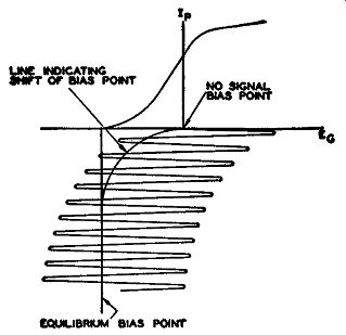
FIG. 8.8. The shift in bias potential during the first few cycles.
Hence, each succeeding cycle of in put voltage will add a little to what remains from the previous cycle. After a few cycles a point of equilibrium is reached and the voltage across R1 remains constant. This establishes the operating bias and the input voltage will fluctuate around this point. The diagram in Fig. 8.8 shows how the tube starts off with zero bias and, after a few cycles, reaches the equilibrium bias point.
The equilibrium bias-point voltage is dependent upon a variety of factors. It depends upon the strength of the input voltage, the voltages on the tube elements, and the time constant of the grid capacitor and resistor. For the latter, the time constant is defined as the time, in seconds, for the capacitor to discharge 63 percent of its voltage through R1. Mathematically, t = RC where R = resistance in ohms, and C = capacitance in farads.
Thus, if we assume values of 0.0001 mf for C and 50,000 ohms for R, we have t=R X C t = 0.0001 X 10^-6 farad X 50,000 ohms t = 5 X 10^-6 second In other words, it requires 5 X 10^-6 second for the charge on the capacitor--no matter what it is-to diminish to 37 percent of its initial value.
Five x 10^-6 second, or 5 microseconds, may not appear to be a very long interval, but it is long if the input wave has a frequency of 100 mhz. At 100 mhz, each cycle requires but 1/100 of a microsecond and 500 input cycles will pass in 5 microseconds.
Time Constant of Limiter Grid-Circuit. The ability of a grid-bias arrangement to remove amplitude variations from the incoming wave depends upon its ability to change its bias as rapidly as the peak amplitude of the incoming wave changes.
For example, suppose the amplitude of the incoming signal suddenly increases. By increasing the bias developed across R1, the grid-leak resistor, correspondingly, it is possible to neutralize the rise in signal amplitude.
The result is then the same as with a smaller signal and a smaller bias.
On the positive peaks, the bias regulates the grid so that it is barely driven positive or just enough to keep the capacitor charged and Eu constant. On the negative peaks, clipping by current cut-off occurs. Thus, by the automatic bias regulation, we can force a constant output for varying inputs.
If a variation in amplitude occurs so rapidly that the bias is unable to change with it, and thus neutralize it, then this change will appear in the output. The ability of the bias to change is a function of the time constant of the grid-leak resistor and capacitor. As we noted previously, with a capacitor of 0.0001 mf value and a resistor of 50,000 ohms, the time constant is 5 microseconds. Compared to the time of. one cycle of a 100 -mhz carrier, an interval of 5 microseconds was long. However, even though the frequency of the incoming signal is 100 mhz, it rarely occurs in practice that each individual cycle will change in amplitude. Hence, we need not make the time constant this low. For most amplitude variations, time constants from 10 to 20 microseconds are more than adequate. The greatest difficulty arises when sharp impulses of the staccato variety, such as we obtain from the ignition system of a car, reach the receiver. If the bias is unable to follow the quick rise and fall of the impulse, a plate current variation will occur and the noise is heard in the speaker. In practice, time constants as low as 1.25 microseconds have been used and the effect of most impulses has been minimized. It must be understood that where the strength of the impulse is greater than the signal, its effect will still be felt. However, the limiter tends to limit the intensity of the impulse and the output noise is not as strong as that of an unobstructed impulse.
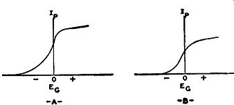
Fig. 8.9. (A) The normal characteristic curve for a sharp cut-off tube.
(B) The modified curve obtained with lowered plate and screen voltage.
Limiting with Low Tube Voltages. The saturation or limiting effect of low plate and screen voltages is best seen by reference to the graphs of Fig. 8.9. In Fig. 8.9A, we have the normal extent of the Eg Ip curve of a sharp cut-off pentode, say, a 6A U6. A sharp cut-off tube is necessary to remove fully the negative ends of the wave. It would be quite difficult to obtain a sharp cut-off in any extended cut-off tube and amplitude variations would be present on the negative peaks of the wave.
When we lower the plate and screen voltages, the extent of the characteristic curve is diminished. This is evident in Fig. 8.9B. It requires much less input signal now to drive the plate current into saturation. An FM receiver having such a limiter would be capable of providing good limiter action with weaker input signals than if the tube were operating with full potentials.
We can, if we wish, operate a tube with lowered electrode potentials only and obtain satisfactory limiting. However, by adding grid-leak bias it is possible to raise somewhat the electrode voltages ( thus providing higher gain) and still obtain good limiting. A typical circuit is in Fig. 8.10.
It was noted previously that, in general, there are two major types of noise which effect a radio wave. One is random or fluctuation noise; the other is the sharp, staccato impulse noise. For the latter type of interference, a low time-constant grid network is best suited to minimize-if not eliminate altogether-the effects of these quick-acting impulses. However, a low valued capacitance and shunt resistance greatly damp the input tuned circuit and consequently lower the effective value of the signal reaching the grid. In order to develop a large signal voltage across a resonant circuit, a high impedance should be presented to that signal. Shunting a low resistance across the circuit reduces the total impedance. In addition, large input signals cause sufficient grid-current flow in the input circuit actually to detune the resonant circuit. With larger time constants, better regulation of the stage is provided.
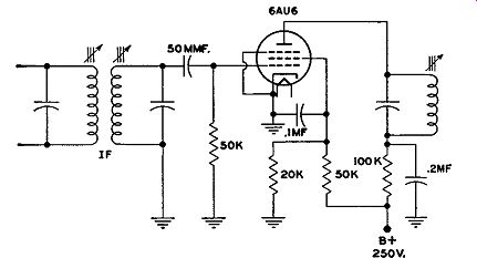
Fig. 8.10. A limiter stage functioning with lowered electrode voltages
and grid leak bias.
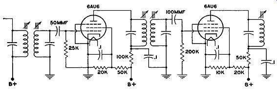
Fig. 8.11. A two-stage (or cascaded) limiter circuit.
Cascaded Limiters. To obtain the advantages that low time constants offer in combating sharp impulses with the better regulation and higher gain of long time-constant networks, some manufacturers have used two limiters in cascade. This is shown in Fig. 8.11. The first limiter has a time constant of 1.25 microseconds. Because of the higher values possible in the second circuit, the gain of both stages averages about 6. With only one stage, values of 2.5 are usual. The increased gain permits the receiver to give full limiter action with weaker input signals.
The advantage can also be seen by reference to the graph of Fig. 8.4.
With two limiters, the knee of the curve is reached by signals of 7 microvolts strength at the receiver input. With one limiter, an input signal of 15 microvolts' strength is required. Any signal weaker than 15 microvolts with one limiter does not give complete limiting action. When the limiter is not operated at saturation, it merely becomes an amplifier and all amplitude noise rides through as readily as the signal itself. This noise is plainly heard at the outer edges of practically all signals or when tuning between stages.
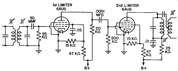
Fig. 8.12. A two-stage resistance-coupled limiter.
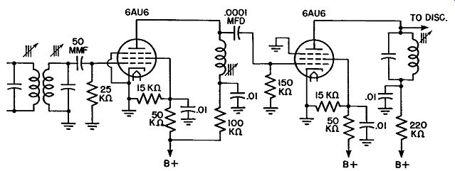
Fig. 8.13. Two limiter stages, impedance-coupled.
Commercial Limiter Circuits. There are two basic limiter circuits in commercial receivers. First, there is the single-stage unit similar to the circuit shown in Fig. 8.10. This functions satisfactorily in sets located near powerful stations where the input signal level is sufficiently strong to provide good limiting. On weak signals, however, noise will be noticeable unless a high degree of amplification is available in the stages preceding the limiter. Cascaded limiters may be either resistance-coupled, as shown in Fig. 8.12, impedance-coupled as in Fig. 8.13, or transformer-coupled. If properly shielded and constructed, the transformer-coupled unit possesses the advantage of an additional voltage gain between circuits, which is not present in the other two circuits. The transformers must be well shielded to prevent feedback and regeneration.
The conventional discriminator is unresponsive to amplitude modulation when the signal is exactly at the center frequency and the circuits are sym metrical. This is true because the discriminator consists of two individual rectifiers which are balanced against each other and the output is the difference between their voltages. At the center frequency, a correctly balanced circuit yields zero output. To obtain full benefit from this feature, however, it is necessary that the resonance point of the discriminator coincide with the resonance points of all the preceding circuits. With strong signals this is difficult to obtain because the large current flow in the grid circuit of the limiter acts to detune the network, and the subsequent loading in the limiter plate circuit produces the same result in the discriminator. However, with strong signals, it is usually possible for the signal to override the noise, and any small distortion introduced because of detuning is generally negligible. With weak signals, however, the effect of noise is correspondingly greater. The advantage to be gained by having the circuits properly aligned at low signal strength is important. It is for this reason that servicing manuals urge alignment with weak generator voltages.
In the choice of a limiter tube, a tube with sharp cut-off characteristics is desirable. In addition, the mutual conductance (gm) should be as high as possible. A large gm will provide more current flow for any given strength of signal and permit the tube to cut-off sharply with smaller input voltages.
EXAM
1. Why are limiters necessary in FM receivers?
2. Do all FM receivers require limiters? Explain.
3. In what section of the FM receiver are limiters placed? Could they be placed elsewhere in the circuit? Explain.
4. Describe the operation of a limiter.
5. How does noise affect the FM signal? Does it affect an AM signal in a similar manner? Why?
6. What advantage do double limiters possess over single limiters?
7. Are limiters always effective in reducing interference? Explain.
8. How much gain can be normally expected from each stage preceding the FM detector? What is the significance of this gain at the limiter? How is the total gain for a receiver computed?
9. Draw the circuit for a grid-leak bias limiter stage.
10. Explain the operation of a grid-leak bias limiter.
11. In what other circuits in radio do we find grid-leak bias?
12. What do we mean by "time constant"? Where is it used? How is it computed?
13. Why is the time constant of the limiter grid circuit important?
14. What effect does the use of lowered voltages have on tube operation?
15. Draw the schematic diagram of a limiter using grid-leak bias and lowered tube voltages. The grid circuit has a time constant of 50 microseconds.
16. Draw the schematic diagram of a two-stage, transformer-coupled limiter circuit. Assign values to all parts, using a 5-microsecond time constant in the grid circuit of the first limiter and a 25-microsecond time constant in the grid circuit of the second limiter.
17. What advantage would a 2-stage transformer-coupled limiter possess over a 2-stage resistance-coupled unit? What disadvantage?
18. Draw the schematic circuit of the I.F. and limiter section of an FM receiver.
Use two I.F. stages and two resistance-coupled limiter stages.
+++++++++++