THERE are a number of ways of measuring the distortion produced in an audio system. Distortion-factor meters and wave analyzers have been used for many years, but intermodulation analyzers are relatively new. Though no objective measurements have yet been devised that can predict accurately whether or not listeners will like the sound of a particular system (the listeners' ears are, after all, the final criterion), intermodulation tests seem to give better clues to hearer acceptance.
Distortion-factor meters are still most common. A single-frequency sine wave is fed into the amplifier and the output is filtered so that the original frequency disappears. The remainder, which consists of any harmonics generated by the amplifier plus whatever noise is present, is measured. The fundamental output is also measured and the harmonics are then figured as a percentage of the fundamental. For good quality systems 5% is often satisfactory, but nowadays high-precision professional and high-fidelity equipment has only a fraction of 1%. The wave analyzer works on the same principle; but instead of measuring all harmonics at once, it filters and measures only one at a time, usually by beating an oscillator with the harmonic to be measured and passing the resultant beat frequency through a very selective filter. The advantage here is that the highly selective filter narrows the bandwidth measured so much that most of the noise is excluded. It also tells just which harmonics are most prominent, giving a clue to the fault, if any, in the system.
The trouble with harmonic measurement is that only distortion in the low-frequency half of the spectrum can be measured; if the fundamental is above the mid-frequency point, all the harmonics fall outside the audio band the equipment covers.
The intermodulation method of measuring distortion is based on the fact that the worst offense to the ears is committed when two or more different frequencies being amplified simultaneously interact due to some nonlinearity in the amplifier. While pure harmonic distortion of a single tone merely creates additional frequencies which are exact multiples of the fundamental, interaction between two or more tones produces sum and difference frequencies which may be totally unrelated harmonically to the originals. The effect is a good deal worse than when some members of a musical ensemble play off pitch or wrong notes, destroying the harmonies or chords. Intermodulation measurements, therefore, usually approximate more closely the subjective reactions of a listener and are generally more useful than simple measurements of spurious harmonics.
The intermodulation method employs two tones: one of low frequency--between about 50 and 200 cycles, and one of considerably higher frequency -anywhere from about 1,000 cycles up. Both tones are fed to an amplifier, and an analyzer connected to the output measures the interaction between them.
The signal generator
Fig. 1001 is a block diagram of a typical intermodulation signal generator. The two oscillators produce sine waves, 60 and 2,000 cycles in this example. (The 60-cycle signal may be provided by the a.c. power line instead of an oscillator.) The two tones are combined in a network carefully designed for minimum distortion.
The resultant wave is shown in Fig. 1001. It is a 2,000-cycle sine wave, with a 60-cycle sine wave as its axis of symmetry. As a more or less standard condition (though no genuine standards have yet been set) the voltage amplitude of the 60-cycle wave is four times that of the 2,000-cycle wave (12 db greater). With this relationship, the inter modulation distortion percentage is usually roughly four times as high as a straight harmonic distortion measurement would be on the same equipment. The exact ratio varies with the cause of distortion.
The output waveform of Fig. 1001 illustrates what happens when ever two or more frequencies are combined--the lower frequencies act as axes for the upper ones, a single composite wave being formed.
The shape, amplitude, and position of any portion of the wave-train about the main a.c. axis depend on the original frequencies, amplitudes, and phase relations. To produce undistorted sound output, the composite wave-train must reach the loudspeaker in exactly the same condition it assumes at the amplifier input. (The exception is that the ear will tolerate a rather large amount of phase change.)
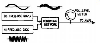
Fig. 1001. Intermodulation signal generator combines two basic frequencies.
As the composite generator output goes through the amplifier being tested, the low-frequency signal causes relatively large positive and negative grid-voltage excursions at each stage. If every tube operates on a linear portion of its transfer characteristic up to the maximum grid-voltage excursions in each direction, no distortion takes place. But if-as is always the case, since nothing is perfect -a nonlinear region is encountered during the swing in one or both directions, those alter nations of the 2,000-cycle superimposed signal which occur while the tube is nonlinear will be either greater or smaller in amplitude than when the tube is operating linearly.
Typical distortion
As an example, suppose one stage in the amplifier is a resistance coupled 6J5 with a 50,000-ohm plate load resistor, a 50,000-ohm following grid resistor, and 1,000-ohm cathode-bias resistor. Plate sup ply voltage is 300. According to the resistance-coupled amplifier charts in the RCA tube manual, voltage gain is 13 and maximum a.c. output voltage should be 41. Dividing 41 by 13, we find that maximum signal voltage at the grid should be 3.15.
Assume that the 3.15-volt input maximum is exceeded slightly. On positive input peaks the grid begins to draw current, flattening off the output wave to some extent. Each time the 60-cycle signal reaches a positive peak, therefore, the amplification of the tube effectively decreases somewhat and the 2,000-cycle alternations superimposed on the 90-degree point of the low-frequency wave have smaller amplitude.
It is likely, too, that negative 60-cycle excursions now take the tube into a nonlinear region, especially with such a low tube-load resistance.
At and about the 270-degree point of the low-frequency wave, there fore, given changes in grid voltage produce smaller changes in plate voltage and again amplification decreases. The result is reduced amplitude of the 2,000-cycle alternations superimposed on the 270-degree region of the 60-cycle wave.
Fig. 1002 is a block diagram of an intermodulation analyzer. The amplifier output wave at A is fed first into a high-pass filter which removes the 60-cycle component from the composite signal. This leaves only the 2,000-cycle signal. Since the amplitude of the 2,000-cycle signal is no longer constant (because of the distortion in the amplifier), it appears at the filter output as a modulated wave (shown at B). Its amplitude is normal or maximum at the points which correspond to the 0-, 180-, and 360-degree regions of the filtered-out 60-cycle wave, and less than normal at the 90- and 270-degree points.
The wave at B is exactly like the familiar r.f. modulated wave (except, of course, for the actual frequency, which is 2,000 cycles) and can be detected and measured in the same way. It is first rectified (detected) to yield the d.c. wave at C. Then it is fed through a low pass filter to remove the 2,000-cycle pulsations. The low-frequency modulation envelope remains at D. Note one important point. The remaining modulation envelope is not the original 60-cycle signal. It is the change in amplitude of the 2,000-cycle signal produced by the 6J5 nonlinearities. Since the amplitude was changed twice during each low-frequency cycle (once by the tube's drawing grid current and once by the negative excursion into a non-linear transfer region), the modulation envelope at D is twice the original low frequency or 120 cycles. If either the negative or positive 6J5 grid excursion alone had caused nonlinearity, that is, a change once per low-frequency cycle, the wave at D would be 60 cycles. Its shape is usually not sine, either, depending on how abruptly the 6J5's characteristic departed from linear.
The wave at D in Fig. 1002 is produced solely by amplifier non linearity, which affected the relationship between two frequencies. If the amplifier were linear, the 2,000-cycle signal would have remained constant in amplitude as it was originally, and detection of a wave at B would have resulted in pure d.c. Obviously, then, the amplitude of the wave at D is a direct indication of the amount of distortion present.
It is measured by an ordinary rectifier-type volt meter. In some instruments, the circuit is arranged so that the operator can tell whether distortion is greater in the negative or positive direction.
The percentage of intermodulation is equal to the modulation percentage of the "carrier" wave at B. With the analyzer calibrated to present a fixed level to the detector, the meter may be marked directly in percent.
When citing intermodulation figures, the test conditions should be specified. The two frequencies should be given, as well as the amplifier output level. For greatest precision, the amplifier input level and the amplitude relationship of the two frequencies should also be mentioned. Measurements should be made with several sets of frequencies, as the distortion varies somewhat.
An amplifier which has low harmonic distortion ordinarily shows low intermodulation as well. Intermodulation results usually agree more closely with listening tests, however, and give a better indication of performance at high frequencies.
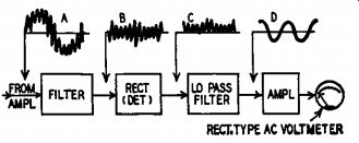
Fig. 1002. The analyzer filters the output signal, detects and measures
distortion.
The percentage figure for intermodulation is always higher than that for harmonic distortion, which is why some manufacturers feel it unwise to publish it. A more valid reason is that standards for inter modulation testing have not yet been agreed on, and this may make interpretation difficult.
Standard intermodulation tests
Two standard intermodulation tests have been advocated. The SMPTE test was standardized by the Society of Motion Picture and Television Engineers. The CCIF test is recommended by the International Telephonic Consultative Committee, and is sometimes called the difference-frequency intermodulation test.
The SMPTE method requires a l.f. and a h.f. test signal. Usually the first is 100 cycles and has 4 times the amplitude of the second which is 5 kc. Due to nonlinearity in the amplifier, sum and difference frequencies are created. They exist as sidebands at intervals of 100 cycles on both sides of the 5-khz "carrier" (see Fig. 1003-a). X and Y are the l.f. and h.f. signals, respectively.
Distortion due to the nth order sideband is then defined by the fraction nth harmonic of sidebands h.f. signal amplitude The CCIF test uses 2 h.f. test signals of equal amplitude. The frequency difference between them is usually in the range 30-400 hertz.
This difference frequency is one of the distortion products due to intermodulation. The distortion it creates is measured by difference-frequency amplitude sum of h.f. test signals
Intermodulation also exists between each h.f. signal and the second harmonic of the other (see Fig. 1003-b). This sideband distortion is de fined by sum of both sidebands / sum of h.f. signals.
According to Peterson*, the CCIF test is better than the SMPTE, especially where the audio system has limited h.f. response. Hearing aids, filters, noise suppressors, etc., are systems that fall in this category.
A harmonic test on them would be misleading because of the limited h.f. response. The SMPTE test cannot give a true picture because it has a strong 1.f. test signal. This means that the h.f. end of the amplifier is not given a real check.
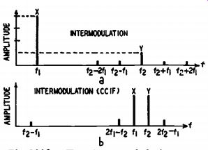
Fig. 1003. Two intermodulation measurement systems. Illustration a is
the SMPTE test. Note the amplitudes of X and Y.
A pair of signal generators are required for intermodulation measurements. For the SMPTE test the frequencies may be fixed at 100 and 5,000 c.p.s. as noted previously. For the difference-frequency test the oscillators may be ganged. This gives a constant beat through a wide range. With this setup X and Y may be moved up and down the scale while (f2-f1) remains stationary (see Fig. 1003-b).
* Arnold P. G. Peterson, Technician. Publication available from General Radio Co.. Cambridge, Mass.