Digital Audio: Speech Coding for Transmission

The purpose of speech coding is to represent speech signals in a format that can be used efficiently for communication. Speech codecs must provide good speech intelligibility, while using signal compression to reduce the bit rate. Although speech codecs have goals that are similar to music codecs, their design is fundamentally different. In particular, unlike music codecs, most speech codecs employ source modeling that tailors the codec to the characteristics of the human voice.

Speech codecs thus perform well with speech signals, and relatively poorly with nonspeech signals. Because most transmission channels have a very limited bit-rate capability, speech coding presents many challenges. In addition to the need to balance speech intelligibility with bit-rate reduction, a codec must be robust over difficult signal conditions, must observe limitations in computational complexity, and must operate with a low delay for real-time communication. Also, wireless systems must overcome the severe error conditions that they are prone to.

Speech Coding Criteria and Overview

A successful speech codec must provide high intelligibility. This includes the ability of the listener to understand the literal spoken content as well as the ability to ascertain the speaker's identity, emotions, and vocal timbre. Beyond intelligible and natural-sounding speech, the speech sound should have a pleasant and listenable quality. Many speech codecs can employ perceptual enhancement algorithms to subjectively improve sound quality. For example, the perception of noise and coding artifacts can be reduced.

Many perceptual enhancements are performed only in the decoder as post-processing. As described later, the performance of speech coding systems can be assessed through subjective listening tests.

A successful speech codec must provide robust performance. A codec should be able to convey speech in the presence of loud background noise and microphone distortion. A codec must provide good performance for different human talkers. For example, the speech sounds of adult males, adult females, and children have very different characteristics. Also, different languages present different coding demands. To a lesser extent, speech codecs should be able to convey nonspeech signals such as dual tone multi-frequency (DTMF) signaling tones and music.

Although fidelity is not expected, the output signal should provide nominal quality. A speech codec should at least be capable of conveying music without overly annoying artifacts.

A speech codec should allow low algorithmic complexity; this directly impacts power consumption and cost. Generally, analysis-by-synthesis techniques are more computationally intensive; thus care must be taken in their design. Other features such as echo cancellation and bandwidth enhancement also add to complexity. From an implementation standpoint, a speech codec should be realizable, and provide good performance, with low computational complexity and low memory size requirements.

A speech codec should introduce minimal delay. All codecs introduce a time delay, the time needed for a signal to enter the encoder and output the decoder. This occurs in the transmission path as algorithmic signal processing (and CPU processing) occurs during encoding and decoding. A codec operating in real time must minimize this coding throughput delay. A coding delay of 40 ms is considered acceptable for speech communications. Low delay codecs may operate with a delay of less than 5 ms.

However, the external communications network may add an additional delay to any signal transmission. Data buffering in the encoder is a primary contributor to delay. Any frame based algorithm incurs finite delay. Speech codecs operate on frames of input samples; for example, 160 to 240 samples may be accumulated (20 ms to 30 ms) before encoding is performed. In most codec designs, greater processing delay achieves greater bit-rate reduction.

Backward-adaptive codecs have an inherent delay based on the size of the excitation frame; delay may be between 1 ms and 5 ms. Forward-adaptive codecs have an inherent delay based on the size of the short-term predictor frame and interpolation; delay may be between 50 ms and 100 ms. In non-real-time applications such as voice mail, coding delay is not a great concern.

As much as possible, a codec must accommodate errors introduced along the transmission channel that may result in clicks or pops. Forward error-correction techniques can provide strong error protection, but may require significant redundancy and a correspondingly higher bit rate. Error-correction coding also introduces overhead data and additional delay.

In many mobile speech transmission systems, unequal error protection (UEP) is used to minimize the effects of transmission bit errors. More extensive error correction is given to high-importance data, and little or no correction is given to low-importance data. This approach is easy to implement in scalable systems (described later), because data hierarchy is already prioritized; core data is protected whereas enhancement-layer data may not be. Sometimes listening tests are used to determine the sensitivity of data types to errors.

A speech coding system is shown in Fig. 1. It contains the same elemental building blocks as the music coding systems described in earlier Sections. For example, the encoder functionally contains a lowpass filter, a sample-and-hold circuit, and an analog-to-digital converter. Similarly, the decoder contains a digital-to analog converter and an output lowpass filter. Historically, telephone systems have provided a narrow audio bandwidth from approximately 300 Hz to 3400 Hz; a sampling frequency of 8 kHz is used. This can allow good intelligibility, while respecting the small signal transmission bandwidth available. As with music coding systems, the coded speech signal is channel-coded to optimize its travel through the transmission channel; for example, error correction processing is applied.

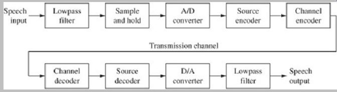
FIG. 1 A speech coding system employs the same general processes as a music coding system. However, the signal coding methods, particularly the codecs employed, are different.

Speech coding for transmission is highly constrained by bit-rate limitations; thus, the transmitted bit rate must be reduced. For example, with an 8-kHz sampling frequency, if 16-bit pulse-code modulation (PCM) words were used, the bit rate input to the source codec would be 128 kbps. However, the speech codec employs lossy coding methods that enable an output bit rate of, for example, 2 kbps to 15 kbps. The speech decoder may use this data-reduced signal to generate a speech signal at the original bit rate, for example, of 128 kbps.

Traditional telephone systems use bit rates such as 64 kbps (PCM) and 32 kbps adaptive differential pulse-code modulation (ADPCM). However, these rates are too high for mobile telephone systems. Simple linear-prediction vocoders may provide a low bit rate of 4 kbps, but speech quality is poor. The bit rate of modern parametric codecs can be quite low, for example, from 2 kbps to 4 kbps, while providing good intelligibility. Many coding systems are scalable; the conveyed bitstream contains embedded lower-rate bitstreams that can be extracted even if the full rate bitstream is not available. In many cases, the embedded bitstreams can be used to improve the sound quality of the base layer bitstream.

As described later, many speech codecs employ a model of the human speech system. The speech system is considered as streams of air passing through the vocal tract. The stream of air from the lungs is seen as a white noise excitation signal. The vocal tract is modeled as a time-varying filter. The output is thus the filter's response to the excitation signal. In particular, as output speech, the signal comprises voiced glottal pulses (modeled as a periodic signal), unvoiced turbulence (modeled as white noise), and a combination of these. At the decoder, the speech signal is reproduced from parameters that represent, from moment to moment, the excitation signal and the filter.

Waveform Coding and Source Coding

Both speech codecs and music codecs have a common goal: to convey an audio signal with the highest possible fidelity and at the lowest possible bit rate. However, their methods are very different. In particular, many speech codecs use a model of the human vocal system, whereas music codecs such as MP3 codecs use a model of the human hearing system.

Many music recording systems use PCM or perceptual coding algorithms such as MP3. These can be classified as waveform codecs because the shape of the music waveform is coded. Among other reasons, this is because the music waveform is highly unpredictable and can take on a wide range of characteristics. Thus, the codec must use a coding approach that can accommodate any possible waveform. Waveform codecs typically represent the waveform as quantized samples or quantized frequency coefficients. Waveform coding requires a relatively higher bit rate to achieve adequate signal quality; for example, a bit rate of 32 kbps may be needed.

ADPCM-algorithms use predictive coding and are used in landline telephone systems. ADPCM is a waveform coding technique and does not use source modeling; thus it can operate equally with voice and music signals.

Compared to other speech codecs that use source modeling, ADPCM is relatively inefficient and uses a relatively high bit rate, for example, from 24 kbps to 32 kbps. Many speech codecs such as ADPCM, particularly in stationary telephone systems, use companding principles.

For example, the µ-law and A-law dynamic compression algorithms use PCM coding and 8-bit word lengths to provide sufficient fidelity for telephone speech communication, as well as bandwidth reduction that is adequate for some applications. In addition, various forms of delta modulation (DM) were sometimes used for speech coding. Delta modulation is a form of predictive coding but does not use source modeling. ADPCM and DM are described in Section 4.

Other speech coding methods provide much greater bandwidth reduction. In particular, they are used in digital mobile telephone systems that require high channel capacity and very low bit rates. These speech coding systems model human speech with speech-specific parameter estimation and also use data compression methods to convey the speech signal as modeled parameters at a low bit rate. The method is somewhat akin to perceptual coding, because there is no attempt to convey a physically exact representation of the original waveform. But in perceptual coding, psychoacoustics is used to transmit a signal that is relevant to the human listener; this is destination coding. In speech coding, speech modeling is used to represent a signal that is based on the properties of the speech source; this is source coding. Source coding is used in mobile (cell) telephones and in Voice over IP (VoIP) applications.

Source encoding and decoding is a primary field of study that is unique to speech coding. Speech codecs are optimized for a particular kind of source, namely a speech signal. Generally speech signals are more predictable than music because the signal always only originates from the human vocal system, as opposed to diverse musical instruments. Thus, speech signals can be statistically characterized by a smaller number of quantized parameters.

Parametric source codecs represent the audio signal with parameters that coarsely describe the characteristics of an excitation signal. These parameters are taken from a model of the speech source. Codec performance is greatly determined by the sophistication of the model. During encoding, parameters are estimated from the input speech signal. A time-varying filter models the speech source, and linear prediction is used to generate filter coefficients.

These parameters are conveyed to the decoder, which uses the parameters to synthesize a representative speech signal. Linear-prediction codecs are the most widely used type of parametric codecs. Because they code speech as a set of parameters extracted from the speech signal rather than as a waveform, speech codecs offer significant data reduction. The bit rate in parametric codecs can be quite low, for example, from 2 kbps to 4 kbps, and can yield good speech fidelity. Because of the nature of the coding technique, higher bit rates do not produce correspondingly higher fidelity.

Hybrid codecs combine the attributes of parametric source codecs and waveform codecs. A speech source model is used to produce parameters that accurately describe the source model's excitation signal. Along with additional parameters, these are used by the decoder to yield an output waveform that is similar to the original input waveform. In many cases, a perceptually weighted error signal is used to measure the difference. Code excited linear prediction (CELP)-type codecs are widely used examples of hybrid codecs. Hybrid codecs typically operate at medium bit rates.

Whereas single-mode codecs use a fixed encoding algorithm, multimode codecs pick different algorithms according to the dynamic characteristics of the audio signal, as well as varying network conditions. Different coding mechanisms are selected either by source control based on signal conditions or by network control based on transmission channel conditions. The selection information is passed along to the decoder for proper decoding.

Although each coding mode may have a fixed bit rate, the overall operation yields a variable bit rate. This efficiency leads to a lower average bit rate.

Human Speech

As noted, speech coding differs from music coding because speech signals only originate from the human vocal system, rather than many kinds of musical instruments. Whereas a music codec must code many kinds of signals, a speech codec only codes one kind of signal. This similarity in speech signals encourages use of source coding in which a model of the human speech system is used to encode and decode the signals. Therefore, an understanding of speech codecs begins with the physiological characteristics and operation of the human vocal tract.

On one hand, speech sounds are easily described. As with all sounds, they are changes in air pressure. Air flow from the lungs is disturbed by constrictions in the body and expelled at the mouth and nostrils. In practice, the human speech system is complex. The formation of speech sounds requires precise control of air flow by many component parts that comprise a time-varying acoustic filter. FIG. 2 shows a simplified view of the human vocal tract. The energy source of the system is the air flow from the diaphragm and lungs. Air flows through the trachea and across the vocal cords (also called vocal folds), a pair of elastic muscle bands and mucous membrane, contained in the larynx, at the "Adam's apple." The vibration of the vocal cords, as they rapidly open and close, forms a noise like excitation signal. The glottis, the opening formed by the vocal cords, can impede air flow and thus cause quasi periodic pulses, or it can allow air to flow freely. When pulses are created, the tension of the vocal cords determines the pitch of the vibration. The velum controls air flow into the nasal cavity. Air flows through the oral and nasal cavities where it is modulated by the tongue, lips, teeth, and jaw, causing localized constriction, and thus changes in air pressure as air passes through. In addition, the oral and nasal cavities act as resonators. The resonant frequencies change according to the position and shape of the vocal tract components. These frequencies are also called formant frequencies.

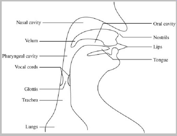
FIG. 2 Representation of the human vocal tract. The system can be modeled in speech codecs as a time varying acoustic filter.

Speech sounds can be considered as voiced or unvoiced. Voiced sounds are formed by spectral shaping of glottal quasi-periodic pulses. In other words, the vibration of the vocal cords interrupts the air flow, creating a series of pulses. Voiced sounds are periodic and thus have a pitch.

The fundamental frequency typically ranges from 50 Hz to 250 Hz for men and from 150 Hz to 500 Hz for women.

Voiced sounds include English-language vowels and some consonants. Unvoiced sounds are not produced by the vocal cords. Rather, they are produced by a steady flow of air passing by stationary vocal cords. The passage through constrictions and other parts of the vocal tract creates aperiodic, noise-like turbulence. Unvoiced sounds include "s" and "f" and "p" sounds. These sounds are also known as fricatives. Sudden releases of air pressure are called stop consonants or plosives; they can be voiced or unvoiced. In addition, transitions from voiced to unvoiced and vice versa are difficult to classify.

Try this experiment: place your fingers on your throat. When making a sustained "aaaaaa" vowel sound, you will feel the vocal-cord vibrations of this voiced sound; moreover, the mouth is open. When making an "mmmmmm" sound, note that it is voiced, but there is no air flow from the closed mouth. Rather, the velum opens so air flows into the nasal cavity to generate a nasal consonant.

When making an "ssssss" sound, note that the vocal cords are silent, and the unvoiced consonant sound comes from your upper mouth. Some sounds, such as a "zzzzzz" sound, are mixed sounds. The beginning of the sustained sound is unvoiced in the upper mouth, followed by voiced vocal-cord vibration. As noted, the place where the constriction occurs will influence the sound. As you say the words, "beet," "bird," and "boot," notice how the vowel sound is formed by the placement of the tongue constriction in the front, middle, and back of the throat, respectively. Similarly, although "p" and "t" and "k" are all plosives, they are created by different vocal tract constrictions: closed lips, tongue against the teeth, and tongue at the back of the mouth. Clearly, even a single spoken sentence requires complex manipulation of the human speech system.

Speech sounds can be classified as phonemes; these are the distinct sounds that form the basis of any language vocabulary. Phonemes are often written with a /*/ notation.

Vowels (for example, /a/ in "father") are voiced sounds formed by quasi-periodic excitation of the vocal cords.

They are differentiated by the amount of constriction, by the position of the tongue, for example, its location from the roof of the mouth, and by lip rounding. Nasal vowels are formed when the velum allows air to the nasal passage.

Fricatives (for example, /s/ in "sap" and /z/ in "zip") are consonants formed by turbulence in air flow caused by constriction in the vocal tract position of the tongue and teeth and lips. They may be voiced or unvoiced. Nasal consonants (for example, /n/ in "no") are voiced consonants where the mouth is closed and the velum allows air flow through the nasal cavity and nostrils. Stop consonants, or plosives (for example, /t/ in "tap" and /d/ in "dip") are formed in two parts: a complete constriction at the lips, behind the teeth or at the rear roof of the mouth, followed by a sudden release of air. They are short-duration transients and affected by the sounds preceding and succeeding them.

They may be voiced or unvoiced. Affricates are a blending of a plosive followed by a fricative. Semivowels (for example, /r/ in "run") are dynamic-voiced consonants. They are greatly affected by the sounds preceding and succeeding them. Diphthongs (for example, /oI / in "boy") are dynamic-voiced phonemes comprised of two vowel sounds. The classification of a sound as a vowel or a diphthong can vary according to regional accents or by individual speakers.

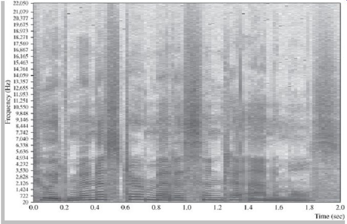
FIG. 3 A spectrogram of the phrase "to administer medicine to animals" spoken by a female talker. Darker areas represent regions of higher signal energy.

Many speech transmission systems convey audio frequencies ranging from 300 Hz to 3400 Hz, and although this is adequate for high intelligibility, human speech actually covers a much wider frequency range. FIG. 3 shows a spectrogram of the phrase "to administer medicine to animals" spoken by a female talker. Darker areas represent regions of higher energy; dark and light banding indicates pitch harmonics. Although the energy in a speech signal is predominantly contained in lower frequencies, there is considerable high-frequency energy.

Source-Filter Model

The source-filter model used in many speech codecs provides an approximation of the human vocal tract, and thus can produce signals that approximate speech sounds.

This design approach is why speech codecs using such a model perform relatively poorly on music signals. The source-filter model is based on the observation that the vocal tract functions as a time-varying filter that spectrally shapes the different sounds of speech. Different speech codecs may use source-filter model approaches that are similar, but the codecs differ in how the speech parameters are created and coded for transmission.

Vocal cords, a fundamentally important source of human speech, are modeled as an excitation signal of spectrally flat sound. The phonemes comprising speech sounds are the result of how this source excitation signal is spectrally shaped by the vocal-tract filter. The excitation signal for voiced sounds (such as vowels) is periodic. This signal is characterized by regularly spaced harmonics (impulses in the time domain). The excitation signal for fricatives (sounds such as "f," "s," and "sh") is similar to Gaussian white noise. The excitation signal for voice fricatives (sounds such as "v" and "z") contains both noise and harmonics.

Channel, Formant, and Sinusoidal Codecs

The channel vocoder, introduced in 1939, was one of the first speech codecs (speech codecs are sometimes referred to as vocoders or voice coders). I t demonstrated that speech could be efficiently conveyed as frequency components. A channel vocoder analysis encoder is shown in Fig. 4A. The input speech signal, considered one frame at a time (for example, 10 ms to 30 ms), is split into multiple frequency bands using fixed bandpass filters. For example, a design may use 20 nonlinearly spaced frequency bands over a 0-Hz to 4-kHz range. Bands may be narrower at lower frequencies. The magnitude of the energy in each subband channel is estimated and output at a low sampling frequency. Further, each frame is marked as voiced or unvoiced. For frames that are voiced, the pitch period is also estimated. Thus, two types of signals are output: magnitude signals and excitation parameters. The magnitude signals can be quantized logarithmically, or the logarithmic difference between adjacent bands can be quantized, for example, using ADPCM coding. Excitation parameters of unvoiced frames may be represented by a signal bit denoting that status. Voiced frames are marked as such, and the pitch period is quantized, for example, with an 8-bit word.

A channel vocoder synthesis decoder is shown in Fig. 4B. The excitation parameters are used to determine the type of excitation signal. For example, unvoiced frames are generated from white noise. Voiced frames are generated from pitch-adjusted harmonic excitation. These sources are applied to each channel and their magnitudes are scaled in each of these subbands. The addition of these subbands produces the speech output. An example of a modern speech vocoder is the version developed by the Joint Speech Research Unit (JSRU). I t uses 19 subbands, codes differences between adjacent subbands, and operates at 24 kbps.

Another type of speech vocoder, a formant speech codec, improves the efficiency of channel vocoders. Rather than code all of the spectral information across the speech frequency band, a formant vocoder only codes the most significant parts. The human vocal tract has several natural resonance frequencies for voiced sounds, called formants.

These are seen as maxima in a spectral envelope; generally there are three significant peaks below 3 kHz. A formant vocoder analysis encoder is shown in Fig. 5A.

The encoder identifies formants on a frame-by-frame basis.

This can be accomplished with formant tracking, that is, by finding the peaks in the spectral envelope. The encoder then codes the formant frequencies and amplitudes. As with channel vocoders, voicing and pitch parameters are also conveyed.

A formant vocoder synthesis decoder is shown in Fig. 5B. The excitation signal is generated based on voicing and pitch parameters, and is used to scale formant amplitude information. This is input to a bank of adjustable bandpass filters that are tuned with formant frequency information and their outputs are summed. Difficulties in formant tracking, such as when spectral peaks do not correlate well with formants, can cause poor performance.

For that reason, formant vocoders are more widely used for speech synthesis where formants are known, rather than for speech coding.

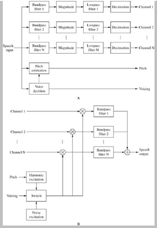
FIG. 4 Channel vocoders convey speech signals as frequency components. A. Channel vocoder analysis encoder. B. Channel vocoder synthesis decoder.

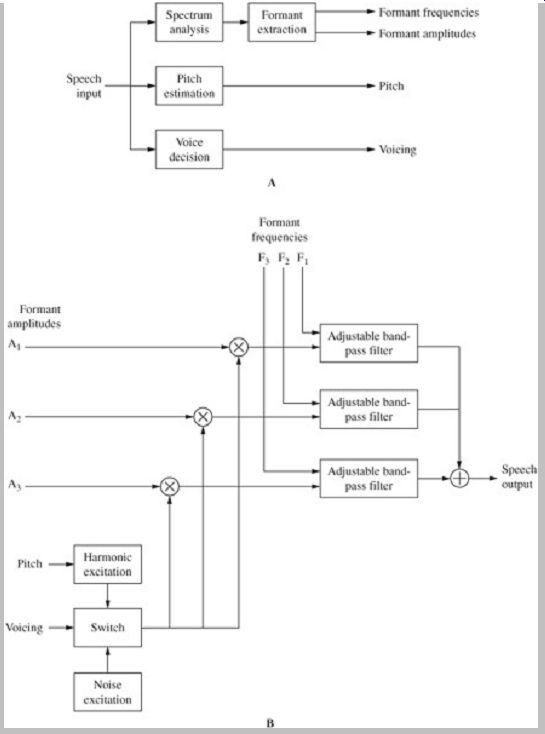
FIG. 5 Formant speech codecs code only the most significant parts of the speech spectrum, natural resonant frequencies called formants. A. Formant vocoder analysis encoder. B. Formant vocoder synthesis decoder.

Sinusoidal speech codecs use sinusoidal modeling to code speech. In this codec, the excitation signal is comprised of the sum of sinusoidal components where amplitude, frequency, and phase are varied to fit the source signal. For example, for unvoiced speech, various sine components with random phases are used. For voiced speech, in-phase, harmonically related sine components, placed at multiples of the pitch frequency, are used. The speech signal input to the encoder can be applied to a Fourier transform; its output can determine the signal peaks. Also, voicing and pitch information are obtained.

Amplitudes are further transformed to the cepstral domain for encoding. At the decoder, the cepstral, voicing and pitch parameters are restored to sinusoidal parameters with an inverse transform, and their amplitudes, frequencies, and phases are used to synthesize the speech output.

Predictive Speech Coding

Speech waveforms are generally simple, being comprised of periodic fundamental frequencies interrupted by bursts of noise. They can be modeled as pulse trains, noise, or a combination of the two. In speech coding, the signal is assumed to be the output response to an input excitation signal. By transmitting parameters that characterize the excitation and vocal-tract effects, the speech signal can be synthesized at the decoder.

The statistics of a speech signal vary over time. In fact, clearly, it is the changes in the signal that convey its information. As one listens to a spoken sentence, the phonemes and frequency content continually change. However, over shorter periods of time, speech signals do not change significantly; thus speech signals are said to be quasi-stationary. Some speech signals, such as vowels, have a very high correlation from sample to sample. For these reasons, many speech codecs operate across short segments of time (perhaps 20 ms or less) and use predictive coding to remove redundancies. With predictive coding, a current input sample value is predicted using values of previously reconstructed samples. The difference between the actual current value and the predicted value is quantized; this is generally more bit-efficient than coding values themselves. The decoder subsequently uses the difference value to reconstruct the signal; this technique is used in ADPCM codecs.

Moreover, at low bit rates, rather than coding the difference signal directly, it is more efficient to code an excitation signal that the decoder can use to synthesize a signal that is close to the original speech signal. This is a characteristic of linear prediction. A short-term predictor describes the spectral envelope of the speech signal while a long-term predictor describes the spectral fine structure.

In some designs (multipulse and regular-pulse excitation), the long-term predictor is omitted or the sequence of the predictors is reversed. An analysis-by-synthesis encoder using short- and long-term prediction is shown in Fig. 6.

Both the long- and short-term predictors are continuously adapted according to the speech signal to improve the efficiency of the prediction; that is, their filter coefficients are changed. The short-term predictor models the vocal tract. Because the vocal tract can only change its physical shape, and hence its output sound, relatively slowly, the parameters can be updated relatively slowly. The short term predictor is often adapted at rates ranging from 30 to 500 times per second. Because an abrupt change in the filter coefficients may produce an audible artifact, values may be interpolated.

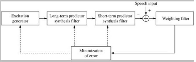
FIG. 6 An analysis-by-synthesis encoder using short-and long-term prediction. Both predictors are continuously adapted according to signal conditions to improve the prediction accuracy.

A long-term prediction filter is generally used to model the periodicity of the excitation signal in code-excited codecs; a small codebook cannot efficiently represent periodicity. A delay might range from 2.5 ms to 18 ms. This accounts for periodicity of pitch from 50 Hz to 400 Hz, which is the range for most human speakers. The coefficients are revised, for example, at rates of 50 to 200 times per second.

Predictor parameters can be determined from a segment (perhaps 10 ms to 30 ms) of the speech signal. In forward-adaptive prediction, the original input speech signal is used, as shown in Fig. 7A. A delay must be used to accumulate the required segment of signal and the parameters are conveyed as part of the output bitstream. In backward-adaptive prediction, the previously reconstructed signal is used to estimate the parameters, as shown in Fig. 7B. Because the reconstructed signal is used, it is not necessary to explicitly convey the parameters in the output bitstream. Either of these methods can be used to estimate the short-term predictor parameters.

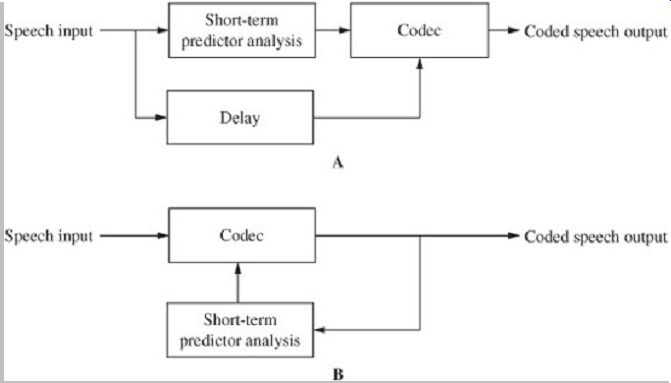
FIG. 7 Either forward- or backward-adaptive methods can be used to determine predictor parameters. A. In forward-adaptive prediction, the original speech signal is used to estimate predictor parameters. B. In backward adaptive prediction, the previously reconstructed signal is used.

The long-term predictor parameters can be estimated using an analysis-by-synthesis method; linear equations are solved for an optimal delay period. Backward-adaptive prediction is not used because the values are sensitive to errors in transmission. Some designs, in place of the long term synthesis filter, use an adaptive codebook that contains versions of the previous excitation. In a code excited codec, the excitation parameters can be determined from the excitation structure and by searching for the codebook sequence to yield the minimal error with the weighted speech signal.

The error between the original and the reconstructed signal can be minimized by using a criterion such the mean-squared error. Except at very low bit rates, this results in a quantization noise that has equal energy at all frequencies. Clearly, low bit rates lead to higher noise levels. The audibility of noise can be minimized by observing masking properties. For example, quantization noise can be spectrally shaped so that its distribution falls within formant peaks in the speech signal's spectral envelope as shown in Fig. 8. Noise shaping can be performed with a suitable error-weighting filter. The mean squared error is increased by noise shaping, but audibility of noise is reduced.

In code-excited or vector-excited codecs, both the encoder and decoder contain a codebook of possible sequences. The encoder conveys an index (the one selected to yield the smallest weighted mean-square error between the original speech signal and the reconstructed signal) to a vector in the codebook. This is used to determine the excitation signal for each frame. The code excited technique is very efficient; an index might occupy 0.2 to 2 bits per sample.

In some cases, a speech enhancement post-filter is used to emphasize the perceptually important formant peaks of the speech signal. This can improve intelligibility and reduce audibility of noise. The post-filter parameters can be derived from the short-term term or long-term prediction parameters. Post-filters introduce distortion and can degrade nonspeech signals.

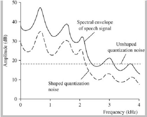
FIG. 8 Noise shaping can be used in a perceptually weighted filter to reduce audibility of noise. The level of shaped noise is equal to that of unshaped noise, but it is less audible.

Linear Predictive Coding

Linear predictive coding (LPC), also referred to as linear prediction, is often used for speech coding. LPC provides an efficient technique for analyzing speech. It operates at a low bit rate and is computationally efficient. It generates estimates of speech parameters using a source-filter model to represent the vocal tract. Linear prediction uses the sum of weighted past time-domain speech signal samples to predict the current speech signal. This inherently reduces the redundancy in the short-term correlation between samples.

In a simple codec, linear prediction can be used in the encoder to analyze the speech signal in a frame, and thus estimate the coefficients of a time-varying filter. These filter coefficients are conveyed along with a scale factor. The decoder generates a white noise signal, multiplies it by the scale factor, and filters it with a filter using the conveyed filter coefficients. This process is updated and repeated for every frame, producing a continuously varying speech signal. Linear prediction is a spectrum estimation technique. Although the output and input signals may differ considerably when viewed in the time domain, the spectrum of the output signal is similar to the spectrum of the original signal. Because the phase differences are not perceived, the output signal sounds similar to the input. Because only the filter coefficients along with a scale factor are conveyed, the bit rate is greatly reduced from the original sampled signal. For example, a frame holding 256 sixteen-bit samples (4096 bits) might be conveyed with 40 bits for the coefficients and 5 bits for the scale factor. In practice, many refinements are applied to this simple codec example to improve its efficiency and performance.

In linear predictive speech codecs, the speech signal is decomposed into a spectral envelope and a residual signal. In some designs, the spectral envelope is represented by LP coefficients (or reflection coefficients). In other designs, the signal is represented by line spectral frequencies (LSFs). The residual signal (error or difference signal) of the LPC encoder can be represented in a variety of ways. LPC codecs use a pulse train and noise representation, ADPCM codecs use a waveform representation. CELP codecs use a codebook representation, and parametric codecs use a parametric representation. Parametric codecs represent the LPC residual signal with harmonic waveforms or sinusoidal waveforms. In particular, the residual signal is conveyed by parametric representation, for example, by sinusoidal harmonic spectral magnitudes. Phase information in the residual is not conveyed. The choice of codec depends on application and bit rate.

Essentially, LPC speech codecs model the human vocal system as a buzzer placed at one end of a tube. More specifically, the model convolves the glottal vibration with the response of the vocal tract. The vocal cords and the space between them, the glottis, produce the buzz which is characterized by changes in loudness and pitch. The throat and mouth of the vocal tract is modeled as a tube; it produces resonances, that is, formants. The tube model works well on vowel sounds but less well on nasal sounds.

The model can be improved by adding a side branch representing the nasal cavity, but this increases computational complexity. In practice, nasal sounds can be accounted for by the residue, as described below.

In LPC the signal is decomposed into two components: a set of LP coefficients and a prediction error (residue) signal. Residual signals are modeled with a pulse train (voiced) or noise (unvoiced); either can be switched in depending on the voicing determination. The coefficients are used in an analysis filter to generate the prediction error signal. The analysis filter has the approximate inverse characteristic of the response of the vocal tract; the prediction error signal acts as the glottal vibration. (voiced) or noise (unvoiced); either can be switched in depending on the voicing determination. The coefficients are used in an analysis filter to generate the prediction error signal. The analysis filter has the approximate inverse characteristic of the response of the vocal tract; the prediction error signal acts as the glottal vibration.

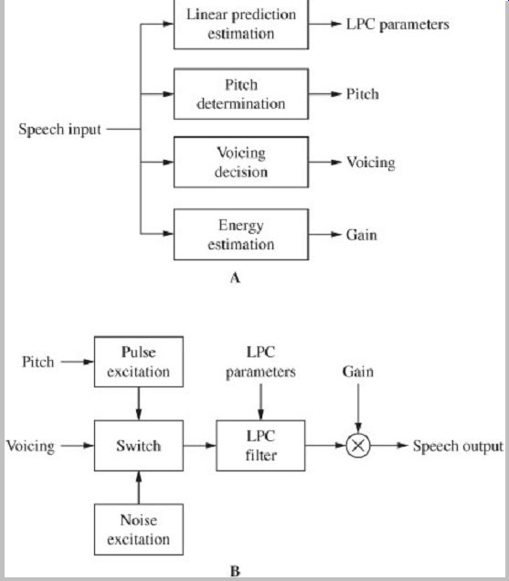
FIG. 9 In linear-predictive coding (LPC) the speech signal is decomposed into a spectral envelope and a residual signal. A. Linear-predictive encoders use a source-filter model to analyze the speech signal. B. Linear predictive decoders reverse the encoding process and synthesize a speech signal.

An LPC encoder is shown in Fig. 9A; four elements are used with a source-filter model to analyze the speech signal. All analysis is done on sampled data segmented into frames. Linear prediction estimates the formants in the spectral envelope and uses inverse filtering to remove their effect from the signal, leaving a residue signal. The encoder then estimates the pitch period and gain of the residue. The frame is classified as voiced or unvoiced using information such as the significance of the harmonic structure of the frame, the number of zero crossings of the time waveform (voiced speech generally has a lower number than unvoiced), or the energy in the frame (voiced speech has higher energy). The formants and residual signal and other information are represented by values that can be stored or transmitted.

An LPC decoder is shown in Fig. 9B; it reverses the encoding process and synthesizes a speech signal. The decoder uses the residue to form a source signal and then uses the formants to filter the source to create speech, thus operating like the original model of the human speech system. The voicing input dictates whether the frame is treated as voiced or unvoiced. When voiced, the excitation signal is periodic and pulses are generated at the proper pitch period. When unvoiced, a random noise excitation is used. In either case, the excitation signal is shaped by the LPC filter and its gain is adjusted to scale the signal amplitude of the output speech.

In the process of estimating speech formants, each signal sample is expressed as a linear combination of previous signal samples. This process uses a difference equation known as a linear predictor (hence the name, linear predictive coding). The process produces prediction coefficients that characterize the formants. The encoder estimates the coefficients by minimizing the mean-square error between the actual input signal and the predicted signal. Methods such as autocorrelation, covariance, or recursive lattice formulation can be used to accomplish this. The process is performed in frames; the frame rate may be 30 to 50 frames per second. Overall bit rate might be 2.4 kbps.

The performance of the LPC technique depends in part on the speech signal itself. Vowel sounds (modeled as a buzz) can be represented as accurate predictor coefficients. The frequency and amplitude of this type of signal can be easily represented. Some speech sounds are produced with turbulent air flow in the human voice system; this hissy sound is found in fricatives and stop consonants. This chaotic sound is different from a periodic buzz. The encoder differentiates between buzz and hiss sounds. For example, for a buzz sound, it may estimate frequency and loudness; for a hiss sound, it may estimate only loudness. For example, the LPC-10e algorithm (found in Federal Standard 1015, described later) uses one value to represent the frequency of buzz, and a value of 0 to signify hiss.

Performance is degraded for some speech sounds that do not fall within the LPC model, for example, sounds that simultaneously contain buzzing and hissing sounds, some nasal sounds, consonants with some tongue positions, and tracheal resonances. Such sounds mean that inaccuracies occur in the estimation of the formants, so more information must be coded in the residue. Good quality can result when this additional information is coded in the residue, but residue coding may not provide adequate data reduction.

As noted, linear predictive encoders generate a residual signal by filtering the signal with an inverse lowpass filter. If this signal was conveyed to the decoder and used as the excitation signal, the speech output would be identical to the original windowed speech signal. However, for this application, the bit rate would be prohibitive. Thus, means are taken to convey the residual signal with a lower bit rate.

The closer the coded residual signal is to the original residual, the better the performance of the codec. The performance of linear predictive coding can thus be improved by using sophisticated (and efficient) means to code the residual signal. In particular, as described later, CELP codecs use codebooks to provide better speech quality than LPC methods, while maintaining a low bit rate.

The Federal Standard 1015, LPC-10e, describes an early, low-complexity LPC codec; it has been superseded by the MELP codec. LPC-10e operates with a frame period of 22.5 ms; with 54 bits per frame, the overall bit rate is 2.4 kbps. It estimates pitch from 50 Hz to 400 Hz using an average magnitude difference function (AMDF); its minima occur at pitch periods for voiced signals. Pitch is coded with 6 bits. Voicing determinations using a linear discriminant classifier are made at the beginning and end of each frame. Factors such as the ratio of AMDF maxima to minima, low-frequency energy content, number of zero crossings, and reflection coefficients are considered in voicing. With voiced speech, low-frequency content is greater than high-frequency content; the first reflection coefficient is used to estimate this. Also in voiced speech, low-frequency peaks are more prominent; the second reflection coefficient estimates this. Tenth-order LPC analysis is used. LPC coefficients are given as log-area ratios for the first two coefficients and as reflection coefficients for the eight higher-order coefficients. Only the first four coefficients (4th order) are coded with unvoiced speech segments while all ten coefficients (10th order) are coded for voiced speech segments.

Code Excited Linear Prediction

The code excited linear prediction (CELP) codec and its variants are the most widely used types of speech codecs.

The CELP algorithm was originally devised by Manfred Schroeder and Bishnu Atal in 1983 and was published in 1985. Originally a particular algorithm, the CELP term now refers to a broad class of speech codecs. Variants of CELP include ACELP, CS-ACELP, RCELP, QCELP, VSELP, FS-CELP, and LD-CELP. CELP-based codecs are used in many mobile phone standards including the Groupe Speciale Mobile (GSM) standard. CELP is used in Internet telephony, and it is the speech codec in software packages such as Windows Media Player. Part of CELP's popularity stems from its ability to perform well over a range of bit rates, for example, from 4.8 kbps (Department of Defense) to 16 kbps (G.728).

The CELP algorithm is based on linear prediction. It principally improves on LPC by keeping codebooks of different excitation signals in the encoder and decoder.

Simply put, the encoder analyzes the input signal, finds a corresponding excitation signal in its code-books, and outputs an indentifying index code. The decoder uses the index code to find the same excitation signal in its codebooks and uses that signal to excite a formant filter (hence the name, code excited linear prediction). As a complete system, CELP codecs combine a number of coding techniques in a novel architecture. As noted, the vocal tract is modeled with a source-filter model using linear prediction, and excitation signals contained in codebooks are used as input to the linear-prediction model. Moreover, the encoder uses a closed-loop analysis by-synthesis search performed in a perceptually weighted domain, and vector quantization is employed to improve coding efficiency.

The heart of the CELP algorithm is shown in Fig. 10.

A codebook contains hundreds of typical residual waveforms stored as code vectors. Codebooks are described in more detail later. Each residual signal corresponds to a frame, perhaps 5 ms to 10 ms, of the original speech signal and is represented by a codebook entry. An analysis-by-syn-thesis method is used in the encoder to select the codebook entry that most closely corresponds to the residual. A codebook outputs a residual signal that undergoes synthesis that is performed in a local decoder contained in the encoder. The selection is performed by matching a code vector-generated synthetic speech signal to the original speech signal; in particular, a perceptually weighted error is minimized.

Clearly, because a codebook is used, there are a finite number of possible residual signals. The decoder contains a gain stage to scale the residual signal, a long-term prediction filter, and a short-term prediction filter. The long term prediction filter contains time-shifted versions of past excitations and acts as an adaptive codebook. The synthesized signal is subtracted from the original speech signal and the difference is applied to a perceptual weighting filter. This sequence is repeated until the algorithm identifies the codebook entry that generates the minimum residual signal. For example, every codebook entry can be sequentially tested. In practice, methods are used to make the codebook search more efficient. The entry yielding the best match is conveyed as the final output. At the receiver, an identical codebook and decoder are used to synthesize the output speech signal.

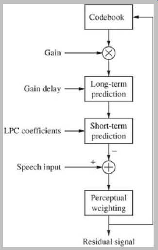
FIG. 10 In the code excited linear prediction (CELP) algorithm, a closed-loop analysis-by-synthesis search is performed in a perceptually weighted domain. The output residual signal is minimized by searching for and selecting the optimal codebook entry.

The final excitation signal is obtained by summing the pitch prediction with an innovation signal from a fixed codebook. The fixed codebook is a vector quantization dictionary that is hard-wired into the codec. The codebook can be stored explicitly (as in Speex) or it can be algebraic (as in ACELP). The innovation signal is the part of the signal that could not be obtained from linear prediction or pitch prediction, and its quantization accounts for most of the allocated bits in a coded signal.

CELP codecs also shape the error (noise) signal so that its energy predominantly lies in frequency regions that are less audible to the ear, thus perceptually minimizing the audibility of noise. For example, the mean square of the error signal in the encoder can be minimized in the perceptually weighted domain. By applying a perceptual noise-weighting filter to the error, the magnitude of the error is greater in spectral places where the magnitude of the speech signal is louder; thus the speech signal can mask the error. The weighting filter can be derived from the linear-prediction coefficients, for example, by using bandwidth expansion. Although far from optimal, the simple weighting filter does improve subjective performance.

In some cases, performance of speech codecs such as CELP is augmented by regenerating additional harmonic content that was lost during coding. In other cases, narrow band coding is improved by estimating a wideband spectral shape from the narrow-band signal. During LPC coding, wideband LPC envelope descriptions are also entered to create a shadow codebook. During decoding, the wideband envelopes are combined with the narrow band excitation.

CELP Encoder and Decoder

The CELP encoder models the vocal tract using linear prediction and an analysis-by-synthesis technique to encode the speech signal. I t accomplishes this by perceptually optimizing the decoded (synthesis) signal in a closed loop. This produces the optimal parameterization of the excitation parameters that are ultimately coded and output by the encoder. When decoded, these yield synthesized speech that best matches the original input speech signal. This kind of perceptually optimized coding may imply that a human listener selects the "best sounding" decoded signal overall. Since this is not possible, the encoder parses the signal into small segments and performs sequential searches using a perceptual-weighting filter in a closed loop that contains a decoding algorithm.

The loop compares an internally generated synthesized speech signal to the original input speech signal. The difference forms an error signal which is iteratively used to update parameters until the closest match is found and the error signal is minimized, thus yielding optimal parameters.

The error signal is perceptually weighted by a filter that is approximately the inverse of the input speech signal spectrum. This reduces the effect of spectral peaks; large peaks would disproportionately influence the error signal and parameter estimation.

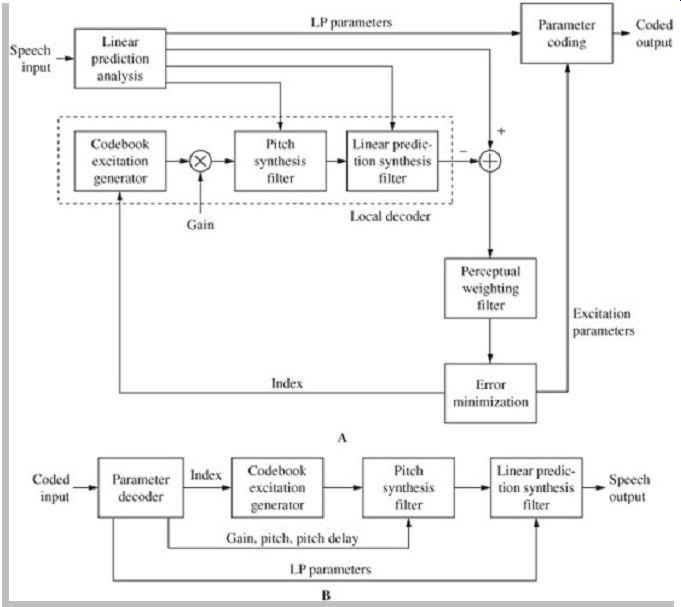
FIG. 11 A CELP encoder and decoder. A. CELP encoders use linear prediction and a local analysis-by synthesis decoder to minimize an error signal and output coding parameters. B. CELP decoders use received parameters to find the corresponding excitation residual and use that signal to excite the formant filter and output the speech signal with a reconstructed LPC filter.

A simplified CELP encoder is shown in Fig. 11A.

The analysis-by-synthesis process begins with an initial set of coding parameters generated by linear-prediction analysis to determine the vocal system's impulse response.

The excitation codebook generator and linear-prediction filter form a local decoder. They output a synthesized speech signal that is subtracted from the original speech input. The difference forms an error signal that is used to improve the parameters by minimizing the perceptually weighted error. The loop iteratively applies the minimized error to the local decoder until its output yields excitation parameters that optimally minimize the energy in the error signal. The parameters are output from the encoder. The LPC parameters are updated for every frame; excitation parameters are updated more often, in subframe intervals.

In some cases, the perceptual-weighting computation is applied to the original input speech signal, rather than to the residual signal. In this way, the computation is performed once, rather than on every loop iteration.

The CELP decoder can be considered as a synthesizer; it uses a speech synthesis technique to output speech signals. A basic CELP decoder is shown in Fig. 11B.

The decoder receives quantized excitation and LPC parameters. Gain, pitch, and pitch delay information is applied to the formant filter. LPC coefficients, representing the vocal tract, are used to reconstruct the linear-prediction filter. The codebook uses the conveyed index code to find the corresponding excitation residuals and uses those signals to excite the formant filter. The output of the formant filter is applied to the linear-prediction filter to generate the output synthesized speech signal. This is done by predicting the input signal using the linear combination of past samples. As with any prediction, there is a prediction error; linear prediction strives to provide the most accurate prediction coefficients and thus minimize the error signal.

The Levinson-Durbin algorithm can be used to perform the computation. Other techniques are used to ensure that the filter is stable.

CELP Codebooks

Linear-predictive encoders such as CELP generate a residual signal. I f this signal were used at the decoder as the excitation signal, the speech output would be identical to the original windowed speech signal. However, the bit rate would be prohibitively high. Thus, the residual signal is coded at a lower bit rate; the closer the coded residual signal is to the original residual, the better the performance of the codec. CELP codecs use codebooks to provide high speech quality, while maintaining a low bit rate.

CELP encoders contain codebooks with tables of pre calculated excitations, each with an identifying index codeword. The encoding analyzer compares the residue to the entries in the codebook table and chooses the entry that is the closest match. I t should provide the lowest quantization error and hence yield perceptually improved coding. The encoder then efficiently sends just the index code that represents that excitation entry. The system is efficient because only a codeword, as well as some auxiliary information, is conveyed.

Testing all of the entries in a large codebook would require considerable computation and time. Much work in CELP design is devoted to minimizing this computational load. For example, codebooks are structured to be more computationally efficient. Also, codewords are altered to reduce the complexity of computation; for example, codewords may be convolved with CELP filters.

Overlapping codebooks are efficient in terms of computation and storage requirements. Rather than store codewords separately, overlapping code-books can store all entries in one array with each codeword value overlapping the next.

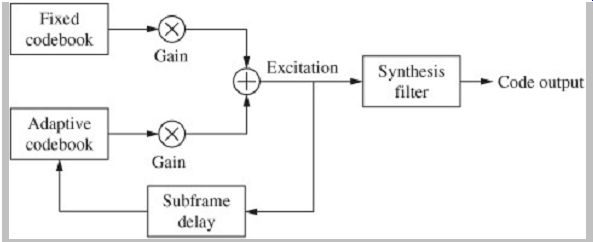
FIG. 12 Both fixed and adaptive codebooks can be used in CELP decoders. Two smaller codebooks can be searched more efficiently than one larger codebook, and their different approaches improve coding performance.

Generally, single-stage codebooks may range in size from 256 (8-bit) to 4096 (12-bit) entries. At least theoretically, performance would be improved if the codebook were large enough to contain every possible residue signal. However, the larger the codebook, the more computation and time required to search it, and the longer the code needed to identify the index. In particular, the codebook would have to contain an individual code for every voice pitch, making the codebook inefficiently large.

Codebooks are generated (trained) using statistical means to improve searching. For example, the LBG clustering algorithm (named after Linde, Buzo, and Gray) is often used to generate codebooks. Beginning with a set of codebook vectors, the algorithm assigns training vectors and recomputes the codebook vectors on the basis of the assigned training vectors. This is repeated until quantization error is minimized.

CELP algorithms can avoid the problem of large codebooks by using two small code-books instead of one larger one. In particular, fixed and adaptive codebooks can be used, as shown in Fig. 12. The fixed (innovation) codebook is set by the algorithm designers and contains the entries needed to represent one pitch period of residue. I t generates signal components that cannot be derived from previous frames; these components are random and stochastic in nature. A vector quantization can be used. In addition to linear prediction, an adaptive (pitch) prediction codebook is used during segments of voiced sounds when the signal is periodic. The adaptive codebook is empty when coding begins, and during operation it is gradually filled with delayed, time-shifted versions of excitations signal coded in previous frames. This is useful for coding periodic signals.

Vector Quantization

Vector quantization (VQ) encodes entire groups of data, rather than individual data points. Analyzing the relationships among the group elements and coding the group is more efficient than coding specific elements.

Moreover, instead of coding samples, VQ systems generally code parameters that define the samples. In the case of speech coding, vector quantization can be used to efficiently code line spectral frequencies that define a vocal tract. VQ is used in CELP and other codecs.

The basic structure of a VQ encoder and decoder is shown in Fig. 13. A speech signal is applied to the encoder. Parameter extraction is performed on a frame basis, for example, with linear-predictive coding to yield parameter vectors. These are compared to vector entries in a fixed, precalculated codebook. A distance metric is used to find the codebook entry that is the best match for the current analyzed vector. The encoder outputs an index codeword that represents the selected codebook entry for that frame.

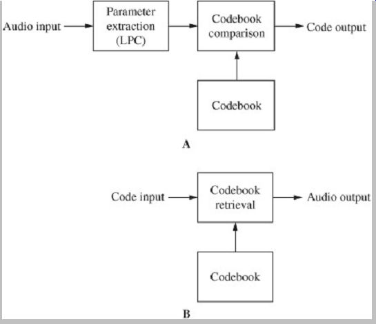
FIG. 13 Vector quantization (VQ) analyzes the parameter relationships among the group elements; coding the group is more efficient than coding specific elements. VQ is used in CELP and other codecs. A. VQ encoder. B. VQ decoder.

The codeword is received by the decoder which contains the same codebook as the encoder. The codeword is used as an index to retrieve the corresponding vector from the codebook. This vector best matches the original vector extracted from the speech signal. This vector is used as the basis for output speech synthesis. For example, voicing and pitch information is also applied.

Examples of CELP Codecs

As noted, many types of CELP codecs are in wide use.

Federal Standard 1016 describes a CELP codec operating at 4.8 kbps. The frame rate is 30 ms with four subframes per frame. The adaptive codebook contains 256 entries; the fixed codebook contains 512 entries. The total delay is 105 ms. The ITU-T G.728 CELP codec operates at 16 kbps; it is designed for low delay (LD) of less than 2 ms. Frame length is 2.5 ms with four subframes per frame. To achieve low delay, only the excitation is conveyed. The fixed codebook coefficients are derived at the decoder using prior decoded speech data. The ITU G.723.1 CELP codec operates at 5.3 kbps and 6.3 kbps; it is used for VoIP and video conferencing. Frame rate is 30 ms with four subframes per frame. Two different codecs are used for the two bit rates, and the system can switch between them on a frame-by-frame basis. Total delay is 37.5 ms. The ETSI GSM Enhanced Full Rate Algebraic CELP codec operates at 12.2 kbps with an additional 10.6 kbps used for error correction; the total bit rate is 22.8 kbps. The codec is used for mobile telephone applications.

The frame rate is 20 ms with five subframes per frame.

Linear-prediction parameters are coded as line spectral pairs (LSPs).

Scalable Speech Coding

Some speech codecs generate embedded (nested) data to allow scalability or other functionality. In addition to core layer data, the conveyed bitstream contains one or more embedded lower-rate bitstreams that can also be extracted and decoded. In many cases, embedded enhancement bitstreams, and their resulting higher bit rate, can be used to improve the sound quality of the core layer bitstream. For example, the embedded layers might reduce coding artifacts or engage a higher sampling frequency to allow a wider audio bandwidth.

A scalable encoder contains a core encoder nested inside enhancement encoders. I t outputs a multi-layer data structure; for example, a three-layer bitstream may contain a core layer and two enhancement layers. The layers are hierarchical; higher layers can only be decoded if lower layers are also received. Using rate adaptation, higher layers may be omitted if dictated by transmission bandwidth or other limitations. The granularity of the coding is determined by the number of layers and increase in bit rate for each layer. The decoder will output a signal that depends on the number of layers transmitted and the capabilities of the decoder.

Scalability allows great diversity in transmission conditions and receiver capability. For example, a VoIP based telecommunications system can choose the appropriate bit-stream according to capacity limitations, while maintaining the best possible sound quality. The technique can also be used to introduce new coding types or improvements while maintaining backward core compatibility. For example, a standard narrow-band codec may comprise the core layer while bandwidth extension uses higher layers.

Scalability can be applied in many different ways. For example, a subband CELP codec may use a QMF filter to split the speech signal into low and high bands. Each band is separately coded with a codec optimized for that frequency range. For example, a CELP codec may be used for the low band and a parameter model codec used for the high band because of reduced tonality of higher frequency signals.

The Internet is a packet-switched network; in contrast to a circuit-switched system, data is formatted and transmitted in discrete data packets. Speech information comprises the payload, and there is also header information. A packet may contain one or more speech frames. In the case of scalable (embedded) VoIP formats, the various layers must be distinguishable and separable.

For example, a packet might contain a single layer; if layers were unneeded, the system could easily drop those packets. However, because of the relatively large amount of header data for each packet (40 to 60 bytes), this approach is inefficient; a speech frame may comprise 80 bytes. A more efficient approach places many speech frames in each packet; this is effective for streaming applications. However, this approach can be sensitive to packet loss, and may incur longer delays. For conversational applications, relatively fewer frames are placed in each packet, and for embedded formats, the various layers are placed in the same packet. For example, if the frame size is approximately 20 ms to 30 ms, one frame can be placed in each packet. The payload would identify the different embedded layers in a frame.

Clearly, the transport protocol must support the data hierarchy and features such as scalability. In addition, the system may prioritize payload data. For example, in the event of network congestion or receiver capability or customer preferences, a rate adaptation unit in the network can transmit core data while dropping enhancement data.

Some data protocol versions such as IPv4 and IPv6 support Differentiated Services. In this case, only complete packets can be labeled, not specific data within. Thus, different layers would be placed in different packets. For example, a scalable MPEG-4 bitstream could be conveyed by multiplexing audio data in Low-overhead MPEG-4 Audio Transport Multiplex (LATM) format and each multiplexed layer is placed in different Real Time Protocol (RTP) packets. In this way, Differentiated Services can distinguish between layers.

G.729.1 and MPEG-4 Scalable Codecs

Scalability features are used in many speech codecs. The ITU-T G.729.1 Voice over IP codec is an example of a scalable codec; it is scalable in terms of bit rate, bandwidth, and complexity. It operates from 8 kbps to 32 kbps, supports 8-kHz and 16-kHz sampling frequency (input and output), and provides an option for lower coding delay. The 8-kbps core codec of G.729.1 provides backward compatibility with the bitstream format of the G.729 codec, which is widely used in VoIP applications.

G.729.1 has two modes: a narrow-band output at 8 kbps and 12 kbps providing an audio bandwidth of 300 Hz to 3400 Hz and a wideband output from 14 kbps to 32 kbps providing an audio bandwidth of 50 Hz to 7000 Hz.

A G.729.1 encoder is shown in Fig. 14A. The input and output sampling frequency is 16 kHz. The encoder uses a QMF analysis filter bank to divide the audio signal into two subbands, split at 4 kHz. The lower band (0-4 kHz) is processed by a 50-Hz high-pass filter and applied to a CELP encoder. The upper band (4-8 kHz) is processed by a 3-kHz lowpass filter and further applied to time-domain bandwidth extension (TDBWE) processing. The upper band signal (prior to TDBWE) and the residual error of the lower-band signal are together applied to a time-domain aliasing cancellation (TDAC) encoder, a transform codec using the modified discrete-cosine transform. Further, frame erasure concealment (FEC) processing is used to generate concealment and recovery parameters used to assist decoding in the presence of frame erasures.

A G.729.1 decoder is shown in Fig. 14B; its operation depends on the bit rate of the received signal. At 8 kbps and 12 kbps, the lower-band signal (50 Hz to 4 kHz) is generated by the CELP decoder and a QMF synthesis filter bank upsamples the signal to a 16-kHz sampling frequency. At 14 kbps, the lower-band 12 kbps signal is combined with a reconstructed higher-band signal from TDBWE processing to form a signal with higher bandwidth (50 Hz to 7 kHz). For received bit rates from 16 kbps to 32 kbps, the upper-band signal and the lower-band residual signal are decoded with TDAC and pre- and post-echo processing reduces artifacts. This signal is combined with the CELP output signal; the TDBWE signal is not used. The decoder can also perform frame erasure concealment using transmitted parameters. As noted, the system can operate in two bit-rate modes: narrow band or wideband.

To avoid audible artifacts when switching between modes, the decoder applies crossfading in the post-filter, and fades in the high band when switching to wideband mode.

The G.729.1 bitstream is hierarchical, enabling scalability. There are 12 layers. The first two layers comprise the narrow-band mode (8 kbps and 12 kbps), and the additional 10 layers comprise the wideband mode (14-32 kbps in steps of 2 kbps). Layer 1 is a core layer (160 bits) that is interoperable with the G.729 format. Layer 2 (12 kbps) is a narrow-band enhancement layer (38 CELP bits and 2 FEC bits) using cascaded CELP parameters and signal class information. Layer 3 (14 kbps) is a wideband extension layer (33 TDBWE bits and 7 FEC bits) with time-domain bandwidth extension parameters and phase information. Layers 4 to 12 (greater than 14 kbps) are wideband extension layers (TDAC1 with 35 TDAC bits and 5 FEC bits, thereafter TDAC2-TDAC9 with 40 TDAC bits) with time-domain aliasing cancellation parameters.

Nominally, the maximum bit rate is 32 kbps; after encoding, the instantaneous bit rate can be set as low as 8 kbps. The frame rate is 20 ms.

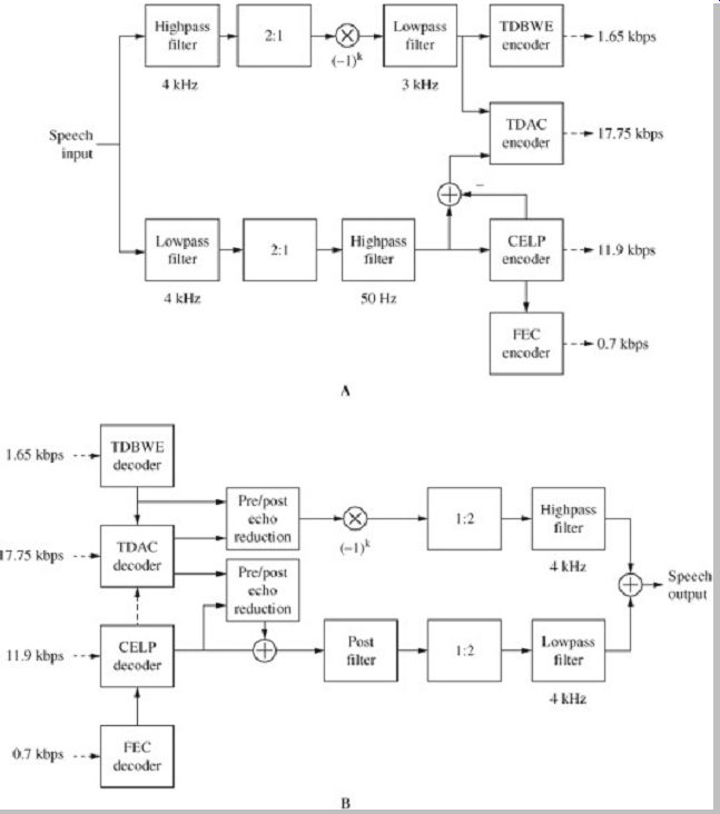
FIG. 14 The ITU-T G.729.1 Voice over IP codec is an example of a scalable codec; it is scalable in terms of bit rate, bandwidth, and complexity. A. G.729.1 encoder. B. G.729.1 decoder.

The G.729.1 codec has a maximum delay of 48.9375 ms; of this, 40 ms is due to TDAC windowing. Delay is reduced in other modes. For example, a delay of 25 ms is possible. Computational complexity varies according to the bit rate. At 32 kbps, total encoder/decoder complexity is 35.8 weighted million operations per second.

Listening evaluations for narrow-band clean speech show that at 8 kbps, G.729.1 has a higher mean opinion score (MOS) than G.729 Annex A, but a lower score than G.729 Annex E. At 12 kbps, the G.729.1 score is more similar to G.729 Annex E. These evaluations are at a 0% frame error rate (FER). At a 6% FER, the 12 kbps G.729.1 scores much higher than Annex A or E. For wideband clean speech, G.729.1 scores higher than G.722.1 at 32 kbps.

For wideband music, at 32 kbps, music quality of G.729.1 is scored similar to G.722.1 at 32 kbps. When comparing codecs, it is important to remember that relative quality varies for different frame-error rates.

Several scalable codecs have been standardized by the Moving Pictures Expert Group of the International Organization for Standardization (ISO/MPEG) and the International Telecommunication Union- Telecommunication Standardization Sector (ITU-T). The MPEG-4 standard (ISO/IEC 14496-3 2005) describes coding tools that can be used for scalable coding. The MPEG-4 CELP codec operates in narrow-band (8-kHz sampling frequency) or wideband mode (16-kHz sampling frequency). In the MPE mode, two types of enhancement layers can be added to the core. In narrow-band mode, the bandwidth is extended, and in wideband mode, the audio signal quality is improved. As another example, the MPEG 4 HVXC narrow-band codec provides a low bit rate of 2 kbps. An optional enhancement layer increases the bit rate to 4 kbps. MPEG-4 is discussed in more detail in Section 15.

Bandwidth Extension

Bandwidth extension (BWE) can be used to improve sound quality in speech codecs. In particular, it supplements the essential data in a narrow-band (NB) signal with additional data. The resulting wideband (WB) signal requires only a modest amount of additional data to greatly extend the frequency range of the audio signal, for example, from a range of 300 Hz to 3400 Hz to a range of 50 Hz to 7000 Hz.

In some cases, the wideband signal is further augmented to produce a super-wideband signal with a high-frequency extension, for example, to 15 kHz. High-frequency extension can improve intelligibility, particularly the ability to distinguish between fricatives (such as "f" and "s" sounds).

Such WB BWE systems can be backward compatible with existing NB systems. Bandwidth extension for speech codecs is similar to spectral band replication techniques used for music signals. One difference is that BWE systems can use signal source models and SBR systems cannot.

Bandwidth extension can be implemented in a number of ways. For example, processing can be placed in both the transmitter (encoder) and receiver (decoder) with transmitted side information (as scalable data) or without (as watermarked data). I t can be placed only in the receiver as post-processing with no transmitted side information. I t can be placed only in the network with a NB/WB transcoder and no transmitted side information.

In bandwidth extension, the parameters of the narrow band signal can be used to estimate a wideband signal. In the case of speech BWE, the estimation can use a speech model similar to the source-filter model used in speech codecs. As noted, speech originates from noise-like signals from the vocal cords and is further processed by the vocal tract and tract cavities. This can be source-modeled with a signal generator and a synthesis filter to shape the spectral envelope of the signal. This model is also used for bandwidth extension; the source component and the filter component are treated separately. The bandwidth of the excitation signal is increased. For example, this can be accomplished with sampling-frequency interpolation, and the narrow-band signal is applied to analysis filters for resynthesis with lower and higher frequencies. Extended frequency harmonics can be generated by distortion or filtering, or by synthetic means, or by mirroring, shifting, or frequency scaling. In addition, feature extraction performed on the narrow-band signal can be used to statistically estimate the spectral envelope. The estimation also incorporates a prior knowledge of both the features and the estimated signal. The spectral envelope is critical in providing improved audio quality. For example, in some systems, only BWE envelope information is transmitted, and excitation extension is only done in the receiver.

FIG. 15 Bandwidth extension (BWE) supplements the essential data in a narrow-band (NB) signal with additional data to produce a wideband (WB) signal. A. Narrow-band encoder with bandwidth extension; BWE information is transmitted as side information. B. Narrow-band decoder with bandwidth extension; the lower subband narrow-band signal is decoded and interpolated to allow addition of the high subband extension.

A narrow-band encoder with bandwidth extension is shown in Fig. 15A. BWE information is transmitted as side information. The speech signal, with a sampling frequency of 16 kHz, is separated into low and high subbands. The lower subband forms the narrow-band signal. I t is decimated to a sampling frequency of 8 kHz and applied to a narrow-band encoder. The higher subband forms the BWE signal. I t is analyzed to determine the spectral and time envelopes (the spectral envelope information may be used in the time-envelope analysis), and quantized BWE parameters are generated. In some cases, a time-envelope prediction residual is transmitted.

A narrow-band decoder with bandwidth extension is shown in Fig. 15B. The lower-subband narrow-band signal is decoded and interpolated to 16 kHz to allow addition of the higher-subband extension. The higher subband BWE parameters are decoded and an excitation signal is generated. This signal is noise-like and may be further refined from parameters from the narrow-band decoder. The subframe time envelope of the excitation signal is shaped by gain factors from the BWE linear prediction decoder. The spectral envelope of the excitation signal is shaped by lowpass filter coefficients from the BWE decoder using an all-pole synthesis filter. The extension signal is added to the narrow-band signal.

In one bandwidth extension implementation that is part of the G.729.1 standard, a FIR filter-bank equalizer is used for spectral envelope shaping in place of a lowpass synthesis filter in the decoder. Filter coefficients are adapted by comparing a transmitted target spectral envelope to the spectral envelope of the synthesized excitation signal, which uses parameters from the narrow band decoder.

Bandwidth extension techniques can also employ watermarking in which the BWE information is hidden in the narrow-band signal. This can promote backward compatibility with narrow-band speech telecommunication systems. As with any watermarking system, the watermark data must not audibly interfere with the host signal. In this case, the BWE data must not degrade intelligibility of the narrow-band signal in receivers that do not make use of the BWE data. Also, its implementation must make the watermark data robust so that it can be conveyed through the complete transmission channel and its associated transcoding, processing, and error conditions. For example, the watermark signal may pass through speech encoding and decoding stages. A system may have unequal error protection. The narrow-band data may have more robust error correction while enhancement layers may have much less. A BWE system must also operate within acceptable computational complexity and latency limits, and the watermark must provide sufficient capacity for useful BWE data.

A watermarking system must analyze the narrow-band host signal to determine how the added watermark can be placed in the signal so the watermark is inaudible.

Perceptual analysis can be used to determine suitable masking properties of the host, or linear prediction can be used to control noise shaping. Techniques such as spread spectrum and dither modulation can be used. Fig. 16A shows a BWE watermark encoder. Operation follows the same steps as any narrow-band encoder. The input speech signal is lowpass filtered and decimated to reduce the sampling frequency to 8 kHz. In a side chain, the input signal is also applied to a BWE encoder, and this information is applied to watermark embedding processing that places the BWE information in the host signal. The embedding process employs analysis of the host signal to modulate and shape the watermarked BWE signal. FIG. 16B shows a BWE watermark decoder. The host narrow-band signal is decoded and interpolated to restore the sampling frequency to 16 kHz. The decoded narrow band signal is applied to a watermark detector. The BWE watermark signal is recovered and decoded, and the high frequency signal components are added to the narrow band signal. I f the watermark signal is not available or properly recovered, the receiver can switch to a separate receiver-only BWE strategy or simply output the narrow band signal without BWE.

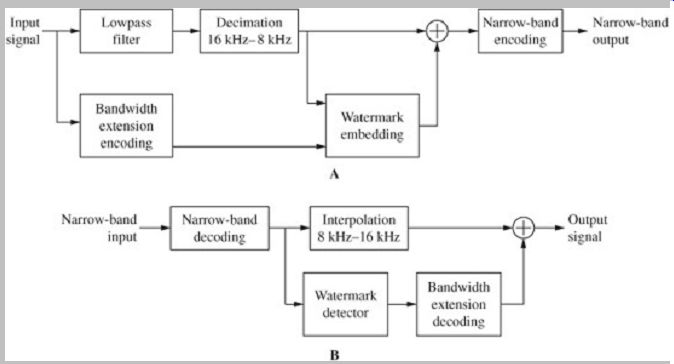
FIG. 16 Bandwidth extension (BWE) techniques can be used in a watermarking system. The system analyzes the narrow-band host signal to determine how the added watermark can be placed in the signal so the watermark is inaudible. A. Speech encoder using watermarked bandwidth extension. B. Speech decoder using watermarked bandwidth extension.

Several WB speech codecs are in use. The G.722.1, introduced in 1999, provides good speech quality at 24 kbps and 32 kbps. The AMR-WB (Adaptive Multi-Rate Wideband) codec, standardized as G.722.2, uses bit rate modes ranging from 6.6 kbps to 23.85 kbps. The AMR WB+ extension uses bit rate modes ranging from 6.6 kbps to 32 kbps and supports monaural and stereo signals, and audio bandwidths ranging from 7 kHz to 16 kHz.

Echo Cancellation

Codec performance can be improved by accounting for distortions such as acoustic echo and background noise.

Echo cancellation addresses a potentially serious issue in speech communication. An acoustic echo is a separately audible delayed reflection from a surface. Acoustic echoes can be produced during hands-free operation, for example, by the acoustic coupling between the loudspeaker and the microphone. Echoes can also be produced electrically. For example, impedance mismatches from hybrid transformers in a long-distance transmission medium can yield line echoes. Both acoustic and electric echoes with long delays can be annoying and can greatly degrade speech intelligibility.

Various techniques have been devised to electrically minimize the effects of echoes. Voice-controlled switching is a simple technique. When a signal is detected at the far speaker side, the microphone signal can be attenuated.

Conversely, during near-end activity, the loudspeaker can be attenuated. However, the result is a half-duplex communication and unnatural changes in noise. The latter can be mitigated by adding comfort noise. Echo suppressors are used to mitigate line echoes using voice operated switches. When an echo is detected (as opposed to an original speech signal), a large loss is switched into the line or the line is momentarily switched open. Errors in operation can occur when the original speech signal's level is low or when the echo signal's level is high.

Adaptive echo cancellation is another approach. Adaptive echo cancelers do not interrupt or alter the communication path. Rather, a synthetic echo is generated from the incoming speech signal, and then later subtracted from the outgoing signal to cancel the echo. Operating in parallel with the actual echo signal path, an adaptive filter uses the known loudspeaker signal to generate a replica of the acoustic echo. The replica echo signal is subtracted from the microphone signal to produce an output speech signal. However, it is difficult to track the original echo path and generate an accurate replica; echo attenuation is insufficient because of a residual echo. Many adaptive algorithms iteratively update filter coefficients using control mechanisms to optimize step size. Some techniques include the delay coefficients method, double-talk detection, remote single-talk detection, two-echo path model, and dynamic regularization. Small steps improve accuracy, but can fail to track changes in the acoustic echo path whereas large steps can cause the algorithm to diverge in noisy conditions. Some designs thus use time varying adaptive step size or adaptive memory. Algorithms include NLMS (normalized least mean square), APA (affine projection), FDAF (frequency domain adaptive filter), and RLS (recursive least square). In some designs, voice controlled switches are combined with echo cancelers. A frequency-selective adaptive post-filter can be used to minimize residual echo after echo cancellation, using the power spectral density of the residual echo. Operation is similar to that of a noise-suppression filter, and in fact noise suppression can be performed simultaneously. Estimation of the residual echo PSD signal is difficult in the context of background noise.

Regarding background noise, for example, a noise signal can be extracted during a pause in speech, and used as a power density spectrum for noise filtering.

Alternatively, during speech, it can be assumed that only noise is present in at least some FFT bins, particularly the lower bins, and the noise power density spectrum can be devised for those bins. To make this determination, for example, it can be assumed that a speech spectrum varies faster than even that of nonstationary noise.

Voice Activity Detection

Voice Activity Detection (VAD) monitors the input signal to determine if the signal is speech or background noise.

When no voice activity and only background noise is detected, the signal is coded with the lowest bit rate needed to convey background noise or a silence compression mode is engaged. During these inactive periods, the decoder may generate a random comfort noise. VAD can be automatically engaged when in variable-bit-rate mode, or engaged separately in constant bit-rate mode. Similarly, when the background noise is stationary, discontinuous transmission (DTX) can be used to halt data transmission, thus further lowering the bit rate.

Variable Bit Rate In some applications such as voice mail, a variable bit rate (VBR) can be used. This can be more efficient than a constant bit rate and can yield a lower average bit rate.

With variable bit rate, a codec can vary its bit rate dynamically according to the nature of the audio signal. A more complex signal demands a higher bit rate, but a less complex signal can be coded with a lower bit rate. Thus, the overall bit rate can be reduced while maintaining an audio quality level. For example, transients and vowels may require a higher bit rate. Fricatives such as "s" and "f" sounds may be coded at a lower bit rate. However, VBR may result in an instantaneous maximum bit rate that is too high. For example, this can overload a real-time channel such as a VoIP channel. Also, when a certain quality level is specified in VBR, a particularly complex audio signal may result in a too-high average bit rate. In many codecs, this problem is addressed by an average-bit-rate (ABR) feature. A target average bit rate is set, and the algorithm monitors and adjusts the variable bit rate to obtain it. This is done in real time with small adjustments. The overall quality of the encoding will be less than would have been obtained with an exactly optimal VBR setting (resulting in the desired average bit rate) without ABR.

Speech Recognition

Many speech recognition systems identify short-term features of speech using cepstral analysis. Other systems may use statistical techniques. In any case, the performance of speech recognition systems can be degraded by poor acoustic conditions such as background noise and room reverberation. In a speech recognition system, the speech signal is applied to front-end processing where short-term spectral analysis is used for feature extraction. In particular, the signal spectrum is transformed to the cepstral domain to obtain the Mel frequency cepstral coefficients. For example, the signal can be pre-emphasized with a highpass filter and input to a Hamming window and FFT to provide a magnitude spectrum. This is applied to a Mel-scale filter bank to emulate critical bands; then the logarithm is taken and this is input to a discrete cosine transform. For example, 13 cepstral coefficients may be calculated including the zeroth coefficient which represents the spectrum mean value. In addition to these short-term static parameters, dynamic parameters may be obtained by examining static contours over several frames. These are sometimes referred to as delta (first derivative) and delta-delta (second derivative) coefficients. For example, a feature vector may contain 39 components; analysis may yield a feature vector every 10 ms. In some cases, the front end is augmented by a noise reduction stage and the cepstral output is applied to blind equalization to yield adaptive equalization.

The output of the cepstral analysis feature extraction stage is used in two modes, as shown in Fig. 17. In the training mode, feature vectors are used to estimate reference patterns that may represent a word or smaller part of speech. Over time, usually with many human talkers, a reference model is assembled and used as a speech pattern database representing the distribution of the characteristics of many human talkers. Hidden Markov models may be used as reference patterns, using sequences of multistate phonemes. In the recognition mode, the input feature vectors are compared to the reference features and the likelihood of correct representation is calculated using a Viterbi or other algorithm. The pattern sequence with the highest likelihood forms the output result.

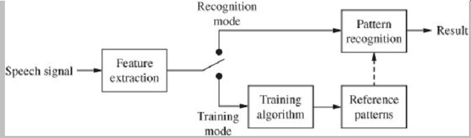
FIG. 17 A speech recognition system showing a training mode, and recognition mode. Short-term spectral analysis can be used for feature extraction.

Speex Codec

The Speex speech codec is used in Voice over IP (VoIP), and streaming applications such as teleconferencing and video games, as well as file-based data reduction applications such as podcasts. I t is not used for cellular telephony. Speex is an open-source codec that can be used freely. Most speech codecs are licensed under patent agreements. Speex is open-source software that does not have any patent or royalty restrictions and can be licensed under the BSD license. Speex shares the same philosophical basis as the Vorbis audio format. Speex was developed by the Xiph.org Foundation; the file name extension is .spx. Speex can be used with the Ogg container format (media type is audio/ogg) or transported directly over UDP/RTP (media type is audio/x-speex).

Speex can be found in DirectShow, OpenACM (NetMeeting), Microsoft Windows, Linux (Ekiga), and libvorbis (Xiph.org's reference implementation).

Speex uses CELP as its coding basis. Among other advantages, this allows Speex to be robust to lost packets, an important consideration for VoIP usage; corrupted packets are blocked from arrival by the User Datagram Protocol (UDP). Speex can be used at different bit rates ranging from 2 kbps to 44 kbps, and at different sampling frequencies including 8 kHz (narrow band), 16 kHz (wideband), 32 kHz (ultra-wideband), and up to 48 kHz.

Narrow band and wideband coding can be contained in the same bitstream. Speex also supports dynamic bit-rate switching, variable bit rate, voice activity detection, and intensity stereo encoding options. In the Speex codec, the delay equals the frame size plus time required to process a frame. This delay is about 30 ms at an 8-kHz sampling frequency and 34 ms at a 16-kHz sampling frequency.

Operation of Speex is controlled by a number of variables. A quality parameter ranges from 0 to 10; this parameter is in integer when in constant-bit-rate (CBR) mode and floating-point number when in variable-bit-rate (VBR) mode. The complexity allowed in the encoder can be varied. To do this, the way that the search is performed is controlled by an integer ranging from 1 to 10 (this is similar to the -1 to -9 options used in gzip compression). Encoder complexity determines CPU requirements; it is about five times higher for a complexity of 10 compared to a complexity of 1. Higher complexities are used for nonspeech signals such as DTMF tones. They are also used when encoding in non-real-time. Generally, a complexity of 2 to 4 is often used.

Quantifying Performance of Speech Codecs

The performance of speech coding systems can be assessed through subjective listening tests. For example, the mean opinion score (MOS) is often used. On this 5 point scale, a score of 4.0 or higher denotes high-quality or near-transparent performance. Scores between 3.5 and 4.0 are often permissible for speech communications systems. Scores below 3.0 denote low quality. For example, a signal may be highly intelligible, but the speech may sound synthetic or otherwise unnatural. A circuit-merit (CM) quality scale can be used to rate subjective performance. The average of CM scores obtained from listeners provides a mean opinion score. The ranking of CM scores is shown in TABLE 1.

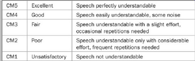
TABLE 1 Ranking of CM scores for subjective performance of speech codecs.

The diagnostic rhyme test (DRT) is a standardized subjective method used to evaluate speech intelligibility. In this American National Standards Institute (ANSI ) test, listeners are presented with word pairs. They must choose which word they perceive. The words are different only in their leading consonants and pairs are selected so that six attributes of speech intelligibility are evaluated in their present or absent states. The diagnostic acceptability measure (DAM) test is also used to evaluate speech codec performance.

Historically, telephone systems provided a narrow bandwidth from approximately 300 Hz to 3400 Hz. I t is generally agreed that the lower cutoff frequency, although it causes a "thin" sound because of missing lower frequencies and thus decreases sound quality, does not greatly affect speech intelligibility. I t is said that the upper cutoff frequency of 3400 Hz allows 97% of speech sounds to be understood. Recognition of sentences can achieve 99% intelligibility because of assistance by context. Newer wideband telephone speech systems provide a response from 50 Hz to 7 kHz. Although the improvement in measured intelligibility is slight, these systems provide a more natural speech sound with clearer sound quality.

Among other things, this suggests the need for more refined telephony sound-quality measures. The subjective evaluation of music signals is discussed in Section 10.

Speech Coding Standards

Speech codecs can be classified as wideband codecs, and narrow-band codecs. Examples of wideband codecs are AMR-WB (for WCDMA networks); VMR-WB (for CDMA2000 networks); and G.722, G.722.1 and Speex (for VoIP and video teleconferencing). Examples of narrow band codecs are SMV (for CDMA networks); Full Rate, Half Rate, EFR, and AMR (for GSM networks); G.723.1, G.726, G.728, G.729, and iLBC (for VoIP and video teleconferencing); and FNBDT (for military applications).

The Telecommunications Industry Association (TIA) has developed speech coding standards for North America including TDMA and CDMA systems. TIA is part of the American National Standards Institute.

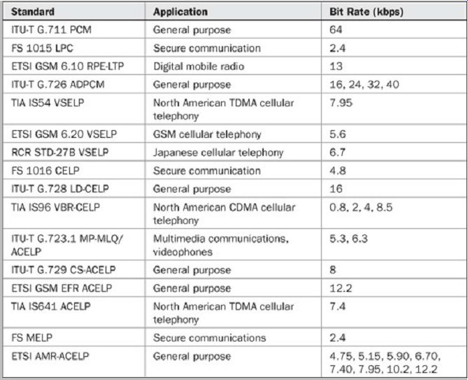
TABLE 2 Summary of speech coding standards.

The G series of International Telecommunications Union (ITU) recommendations define speech coding standards including G.711 (µ law), G.728 (LD-CELP), and G.729A (CS-ACELP).

The European Telecommunications Standards Institute (ETSI ) publishes standards for digital cellular applications in Europe. The Groupe Speciale Mobile (GSM) has developed standards such as GSM 06.60 and 06.90.

The International Standards Organization (ISO) contains the Moving Picture Experts Group (MPEG). The MPEG 4 standard describes the Harmonic Vector Excitation (HVXC) codec and narrow-band and wideband CELP codecs.

The U.S. Department of Defense Voice Processing Consortium (DDVPC) standardized the Federal Standard FS1015 LPC-10e and FS1016 CELP codecs, as well as the MELP and MELPe MIL-STD-3005 standard, adopted as the STANAG-4591 standard.

The Research and Development Center for Radio Systems of Japan (RCR) develops digital cellular standards for Japan.

A list of some speech coding standards is shown in TABLE 2.

Prev. | Next

Top of Page   All Related Articles    Home