The digital techniques used to record, reproduce, store, process, and transmit digital audio signals entail concepts foreign to analog audio methods. In fact, the inner workings of digital audio systems bear little resemblance to analog systems. Because audio itself is analog in nature, digital systems employ sampling and quantization, the twin pillars of audio digitization, to represent the audio information.
Any sampling system is bound by the sampling theorem, which defines the relationship between the message and the sampling frequency. In particular, the theorem dictates that the message be bandlimited. Precaution must be taken to prevent a condition of erroneous sampling known as aliasing. Quantization error occurs when the amplitude of an analog waveform is represented by a binary word; effects of the error can be minimized by dithering the audio waveform prior to quantization.
Discrete Time Sampling
With analog recording, a tape is continuously modulated or a groove is continuously cut. With digital recording, discrete numbers must be used. To create these numbers, audio digitization systems use time sampling and amplitude quantization to encode the infinitely variable analog waveform as amplitude values in time. Both of these techniques are considered in this Section . First, let's consider discrete time sampling, the essence of all digital audio systems.
Time seems to flow continuously. The hands of an analog clock sweep across the clock face covering all time as it passes by. A digital readout clock also tells time, but with a discretely valued display. In other words, it displays sampled time. Similarly, music varies continuously in time and can be recorded and reproduced either continuously or discretely. Discrete time sampling is the essential mechanism that defines a digital audio system, permits its analog-to-digital (A/D) conversion, and differentiates it from an analog system.
However, a nagging question immediately presents itself. If a digital system samples an audio signal discretely, defining the audio signal at distinct times, what happens between samples? Haven't we lost the information present between sample times? The answer, intuitively surprising, is no. Given correct conditions, no information is lost due to sampling between the input and output of a digitization system. The samples contain the same information as the conditioned unsampled signal. To illustrate this, let's try a conceptual experiment.
Suppose we attach an iPhone (camera, at 24- or 30-fps) to the handlebars of a bicycle, go for a ride. Auditioning this piece of avant-garde cinema, we discover that the discrete frames off video reproduce our ride. But when we traverse bumpy pavement, the picture is blurred. We determine that the quick movements were too fast for each frame to capture the change. We draw the following conclusion: if we increased the frame rate, using more frames per second, we could capture quicker changes. Or, if we complained to city hall and the bumpy pavement was smoothed, there would be no blur even at slower frame rates. We settle on a compromise--we make the roads reasonably smooth, and then we use a frame rate adjusted for a clean picture.
The analogy is somewhat clumsy. (For starters, cinema comprises a series of discontinuous still images-it is the brain itself that creates the illusion of a continuum. An audio waveform played back from a digital source really is continuous because of the interpolation function used to create it.) Nevertheless, the analogy shows that the discrete frames of a movie create a moving picture, and similarly the samples of a digital audio recording create a continuous signal. As noted, sampling is a lossless process if the input signal is properly conditioned. Thus, in a digital audio system, we must smooth out the bumps in the incoming signal. Specifically, the signal is low pass filtered; that is, the frequencies that are too high to be properly sampled are removed. We observe that a signal with a finite frequency response can be sampled without loss of information; the samples contain all the information contained in the original signal. The original signal can be completely recovered from the samples. Generally, we observe that there exists a method for reconstructing a signal from its amplitude values taken at periodic points in time.
The Sampling Theorem
The idea of sampling occurs in many disciplines, and the origin of sampling theorems comes from many sources.
Most audio engineers recognize American engineer Harry Nyquist as the author of the sampling theorem that founded the discipline of modern digital audio. The recognition is well-founded because it was Nyquist who expressed the theorem in terms that are familiar to communications engineers. Nyquist, who was born in Sweden in 1889, and died in Texas in 1976, worked for Bell Laboratories and authored 138 U.S. patents. However, the story of sampling theorems predates Nyquist.
When he was not busy designing military fortifications for Napoleon, French mathematician Augustin-Louis Cauchy contemplated statistical sampling. In 1841, he showed that functions could be nonuniformly sampled and averaged over a long period of time. At the turn of the century, it was thought (incorrectly) that a function could be successfully sampled at a frequency equal to the highest frequency. In 1915, Scottish mathematician E. T. Whittaker, working with interpolation series, devised perhaps the first mathematical proof of a general sampling theorem, showing that a band-limited function can be completely reconstructed from samples. In 1920, Japanese mathematician K. Ogura similarly proved that if a function is sampled at a frequency at least twice the highest function frequency, the samples contain all the information in the function, and can reconstruct the function. Also in 1920, American engineer John Carson devised an unpublished proof that related the same result to communications applications.
It was Nyquist who first clarified the application of sampling to communications, and published his work. In 1925, in a paper titled "Certain Factors Affecting Telegraph Speed," he proved that the number of telegraph pulses that can be transmitted over a telegraph line per unit time is proportional to the bandwidth of the line. In 1928, in a paper titled "Certain Topics in Telegraph Transmission Theory," he proved that for complete signal reconstruction, the required frequency bandwidth is proportional to the signaling speed, and that the minimum bandwidth is equal to half the number of code elements per second.
Subsequently, Russian engineer V. A. Kotelnikov published a proof of the sampling theorem in 1933.
American mathematician Claude Shannon unified and proved many aspects of sampling, and also founded the larger science of information theory in his 1948 book, A Mathematical Theory of Communication. Shannon's 1937 master's thesis, "A Symbolic Analysis of Relay and Switching Circuits," showed that circuits could use Boolean algebra to solve logical or numerical problems; his work was called "possibly the most important, and also the most famous, master's thesis of the century." Shannon, a distant relative of Thomas Edison, could also juggle three balls while riding a unicycle. Today, engineers usually attribute the sampling theorem to Shannon or Nyquist. The half sampling frequency is usually known as the Nyquist frequency.
Whoever gets the credit, the sampling theorem states that a continuous band limited signal can be replaced by a discrete sequence of samples without loss of any information and describes how the original continuous signal can be reconstructed from the samples; furthermore, the theorem specifies that the sampling frequency must be at least twice the highest signal frequency. More specifically, audio signals containing frequencies between 0 and S/2 Hz can be exactly represented by S samples per second. Moreover, in general, the sampling frequency must be at least twice the bandwidth of a sampled signal. When the lowest frequency of the bandwidth of interest is zero, then the signal's bandwidth equals the highest frequency.
The sampling theorem is applied widely and diversely throughout engineering, science, and mathematics.
Nyquist Frequency
When the sampling theorem is applied to audio signals, the input audio signal is low-pass filtered, so that it’s band limited with a frequency response that does not exceed the Nyquist (S/2) frequency. Ideally, the low pass filter is designed so that the only signals removed are those high frequencies that lie above the high-frequency limit of human hearing. The signal can now be sampled to define instantaneous amplitude values. The sampled band limited signal contains the same information as the unsampled band limited signal. At the system output, the signal is reconstructed, and there is no loss of information (due to sampling) between the output signal and the input filtered signal. From a sampling standpoint, the output signal is not an approximation; it’s exact. The band limited signal is thus re-created, as shown in Fgr. 1.
Consider a continuously changing analog function that has been sampled to create a series of pulses. The amplitude of each pulse, determined through quantization, yields a number that represents the signal amplitude at that instant. To quantify the situation, we define the sampling frequency as the number of samples per second. Its reciprocal, sampling rate, defines the time between each sample. For example, a sampling frequency of 48,000 samples per second corresponds to a rate of 1/48,000 seconds. A quickly changing waveform-that is, one with high frequencies-requires a higher sampling frequency.
Thus, the digitization system's sampling frequency determines the high frequency limit of the system. The choice of sampling frequency is thus one of the most important design criteria of a digitization system, because it determines the audio bandwidth of the system.
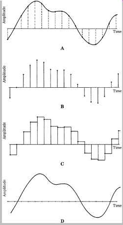
FGR. 1 With discrete time sampling, a bandlimited signal can be sampled and
reconstructed without loss because of sampling. A. The input analog signal
is sampled. B. The numerical values of these samples are stored or transmitted
(effect of quantization not shown). C. Samples are held to form a staircase
representation of the signal. D. An output lowpass filter interpolates the
staircase to reconstruct the input waveform.
The sampling theorem precisely dictates how often a waveform must be sampled to provide a given bandwidth.
Specifically, as noted, a sampling frequency of S samples per second is needed to completely represent a signal with a bandwidth of S/2 Hz. In other words, the sampling frequency must be at least twice the highest audio frequency to achieve lossless sampling. For example, an audio signal with a frequency response of 0 to 24 kHz would theoretically require a sampling frequency of 48 kHz for proper sampling. Of course, a system could use any sampling frequency as needed. It’s crucial to observe the sampling theorem's criteria for limiting the input signal to no more than half the sampling frequency (the Nyquist frequency). An audio frequency above this would cause aliasing distortion, as described later in this Section . A lowpass filter must be used to remove frequencies above the half-sampling frequency limit. A lowpass filter is also placed at the output of a digital audio system to remove high frequencies that are created internally in the system.
This output filter reconstructs the original waveform.
Reconstruction is discussed in more detail in Section 4.
Another question presents itself with respect to the sampling theorem. We observe that when low audio frequencies are sampled, because of their long wavelengths, many samples are available to represent each period. But as the audio frequency increases, the periods are shorter and there are fewer samples per period. Finally, in the theoretical limiting case of critical sampling, at an audio frequency of half the sampling frequency, there are only two samples per period. However, even two samples can represent a waveform. For example, consider the case of a 48-kHz sampling frequency and an audio input of 24-kHz sine wave. The sampler produces two samples, which will yield a 24-kHz square wave. In itself, this waveform is quite unlike the original sine wave.
However, a lowpass filter at the output of the digital audio system removes all frequencies higher than the half sampling frequency. (The 24-kHz square wave consists of odd harmonics-sine waves starting at 24 kHz.) With all higher frequency content removed, the output of the system is a reconstructed 24-kHz sine wave, the same as the sampled waveform. We know that the sampled waveform was a sine wave because the input lowpass filter won’t pass higher waveform frequencies to the sampler.
Similarly, a digitization system can reproduce all information from 0 to S/2 Hz, including sine wave reproduction at S/2 Hz; even in the limiting case, the sampling theorem is valid. Conversely, all information above S/2 is removed from the signal. We can state that higher sampling frequencies permit recording and reproduction of higher audio frequencies. But given the design criteria of an audio frequency bandwidth, higher sampling frequencies won’t improve the fidelity of those signals already within the bandlimited frequency range.
For critical sampling, there is no guarantee that the sample times will coincide with the maxima and minima of the waveform. Sample times could coincide with lower amplitude parts of the waveform, or even coincide with the zero-axis crossings of the waveform. In practice, this does not pose a problem. Critical sampling is not attempted; a sampling margin is always present. As we have seen, to satisfy the sampling theorem, a lowpass filter must precede the sampler. Lowpass filters cannot attenuate the signal precisely at the Nyquist frequency so a guard band is employed. The filter's cutoff frequency characteristic starts at a lower frequency , for example, at 20 kHz, allowing several thousand Hertz for the filter to attenuate the signal sufficiently. This ensures that no frequency above the Nyquist frequency enters the sampler. The waveform is typically not critically sampled; there are always more than two samples per period. Furthermore, the phase relationship between samples and waveforms is never exact because acoustic waveforms don’t synchronize with a sampler. Finally, when we examine the sampling theorem more rigorously in Section4, we will see that parts of the waveform lying between samples can be captured and reproduced by sampling. We shall see that the output signal is not reconstructed sample by sample; rather, it’s formed from the summation of the response of many samples. It’s also worth noting that the bandwidth of any practical analog audio signal is also limited. No analog audio system has infinite bandwidth. The finite bandwidth of audio signals shows that the continuous waveform of an analog signal or the samples of a digital signal can represent the same information.
The need to bandlimit the audio signal is not as detrimental as it might first appear. The upper frequency limit of the audio signal can be extended as far as needed, so long as the appropriate sampling frequency is employed. For example, depending on the application, sampling frequencies from 8 kHz to 192 kHz may be used.
The trade-off, of course, is the demand placed on the speed of digital circuitry and the capacity of the storage or transmission medium. Higher sampling frequencies require that circuitry operate faster and that larger amounts of data be conveyed. Both are ultimately questions of economics.
Manufacturers selected a sampling frequency of 44.1 kHz for the Compact Disc , for example, because of its size, playing time, and cost of the medium. On the other hand, DVD-Audio and Blu-ray discs can employ sampling frequencies up to 192 kHz.
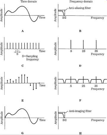
FGR. 2 Time domain (left column) and frequency domain (right column) signals
illustrate the process of bandlimited waveform sampling and reconstruction.
A.
Input signal after anti-aliasing filter. B. Spectrum of input signal. C. Sampling signal. D. Spectrum of the sampling signal. E. Sampled input signal. F. Spectrum of the sampled input signal. G. Output signal after anti-imaging filter. H. Spectrum of the output signal.
The entire sampling (and desampling) process is summarized in Fgr. 2. The signals involved in sampling are shown at different points in the processing chain.
Moreover, the left half of the figure shows the signals in the time domain and the right half portrays the same signals in the frequency domain. In other words, we can observe a signal's amplitude over time, as well as its frequency response. We observe in Fgrs. A and B that the input audio signal must be bandlimited to the half-sampling frequency S/2, using a lowpass anti-aliasing filter. This filter removes all components above the Nyquist frequency of S/2. The sampling signal in Fgrs. C and D recurs at the sampling frequency S, and its spectrum consists of pulses at multiples of the sampling frequency: S, 2S, 3S, and so on. When the audio signal is sampled, as shown in Figs. 2E and F, the signal amplitude at sample times is preserved; however, this sampled signal contains images of the original spectrum centered at multiples of the sampling frequency. To reproduce the sampled signal, as in Fgrs. 2G and H, the samples are passed through a lowpass anti-imaging filter to remove all images above the S/2 frequency. This filter interpolates between the samples of the waveform, recreating the input, bandlimited audio signal. As described in Section 4, the output filter's impulse response uniquely reconstructs the sample pulses as a continuous waveform.
The sampling theorem is unequivocal: a bandlimited signal can be sampled; stored, transmitted, or processed as discrete values; desampled; and reconstructed. No band-limited information is lost through sampling. The reconstructed waveform is identical to the bandlimited input waveform. Sampling theorems such as the Nyquist theorem prove this conclusively. Of course, after it has time-sampled the signal, a digital system also must determine the numerical values it will use to represent the waveform amplitude at each sample time. This question of quantization is explained subsequently in this Section . For a more detailed discussion of discrete time sampling, and a concise mathematical demonstration of the sampling theorem, refer to the Wikipedia .
Aliasing
Aliasing is a kind of sampling confusion that can originate in the recording side of the signal chain. Just as people can take different names and thus confuse their identity, aliasing can create false signal components. These erroneous signals can appear within the audio bandwidth and are impossible to distinguish from legitimate signals.
Obviously, it’s the designer's obligation to prevent such distortion from ever occurring. In practice, aliasing is not a serious limitation. It merely underscores the importance of observing the criteria of the sampling theorem.
We have observed that sampling is a lossless process under certain conditions. Most important, the input signal must be bandlimited with a lowpass filter. If this is not done, the signal might be undersampled. Consider another conceptual experiment: use your motion picture camera to film me while I drive away on my motorcycle. In the film, as I accelerate, the spokes of the wheels rotate forward, appear to slow and stop, then begin to rotate backward, rotate faster, then slow and stop, and appear to rotate forward again. This action is an example of aliasing. The motion picture camera, with a frame rate of 24 frames per second, cannot capture the rapid movement of the wheel spokes.
Aliasing is a consequence of violating the sampling theorem. The highest audio frequency in a sampling system must be equal to or less than the Nyquist frequency. If the audio frequency is greater than the Nyquist frequency, aliasing will occur. As the audio frequency increases, the number of sample points per period decreases. When the Nyquist frequency is reached, there are two samples per period, the minimum needed to record the audio waveform.
With higher audio frequencies, the sampler will continue to produce samples at its fixed rate, but the samples create false information in the form of alias frequencies. As the audio frequency increases, a descending alias frequency is created. Specifically, if S is the sampling frequency, F is a frequency higher than the half-sampling frequency, and N is an integer, then new frequencies Ff are created at Ff = ± NS ± F.
In other words, alias frequencies appear back in the audio band (and the images of the audio band), folded over from the sampling frequency. In fact, aliasing is sometimes called foldover. Although disturbing, this is not totally surprising. Sampling is a kind of modulation; in fact, sampling is akin to the operation of a hetero-dyne demodulator in an amplitude modulation (AM) radio. A local oscillator multiplies the input signal to move its frequency down to the standard intermediate frequency (IF).
Although the effect is desirable in radios, aliasing in digital audio systems is undesirable.
Consider a digitization system sampling at 48 kHz.
Further, suppose that a signal with a frequency of 40 kHz has entered the sampler, as shown in Fgr. 3. The primary alias component results from S - F = Ff or 48 - 40 = 8 kHz.
The sampler produces the improper samples, faithfully recording a series of amplitude values at sample times.
Given those samples, the device cannot determine which was the intended frequency: 40 kHz or 8 kHz. Furthermore, recall that a lowpass filter at the output of a digitization system smoothes the staircase function to reconstruct the original signal. The output filter removes content above the Nyquist frequency. In this case, following the output filter, the 40-kHz signal would be removed, but the 8-kHz alias signal would remain, containing samples as innocuous as a legitimate 8-kHz signal. That unwanted signal is a distortion in the audio signal.
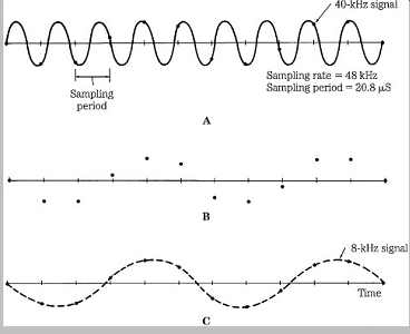
FGR. 3 An input signal greater than the half-sampling frequency will generate
an alias signal, at a lower frequency. A. A 40-kHz signal is sampled at 48
kHz. B. Samples are saved. C. Upon reconstruction, the 40-kHz signal is filtered
out, leaving an aliased 8-kHz signal.
There are other manifestations of aliasing. Although only the S - F component appears as an interfering frequency in the audio band, an alias component will appear in the audio band, no matter how high in frequency F becomes.
Consider a sampling frequency of 48 kHz; a sweeping input frequency from 0 to 24 kHz would sound fine, but as the frequency sweeps from 24 kHz to 48 kHz, it returns as a frequency descending from 24 kHz to 0. If the input frequency sweeps from 48 kHz to 72 kHz, it appears again from 0 to 24 kHz, and so on.
Alias components occur not only around the sampling frequency, but also in the multiple images produced by sampling (see Fgr. 2F). When the sampling theorem is obeyed, the audio band and image bands are separate, as shown in Fgrs. 4A and B. However, when the audio band extends past the Nyquist frequency, the image bands overlap, resulting in aliasing as shown in Fgrs. 4C and D.
All these components would be produced in an aliasing scenario: ± S ± F, ± 2S ± F, ± 3S ± F, and so on. For example, given a 48-kHz sampler and a 29-kHz input signal, some of the resulting alias frequencies would be 19, 67, 77, 115, 125, 163, and 173 kHz, as shown in Fgr. 4D.
With a sine wave, aliasing is limited to the one and only partial of a sine wave. With complex tones, content is generated for all spectra above the Nyquist frequency.
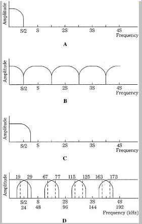
FGR. 4 Spectral views of correct sampling and incorrect sampling causing
aliasing. A. An input signal bandlimited to the Nyquist frequency. B. Upon
reconstruction, images are contained within multiples of the Nyquist frequency.
C. An input signal that is not bandlimited to the Nyquist frequency. D. Upon
reconstruction, images are not contained within multiples of the Nyquist frequency;
this spectral overlap is aliasing; For example, a 29-kHz signal will alias
in a 48-kHz sampler.
In practice, aliasing can be overcome. In fact, in a properly designed digital recording system, aliasing does not occur. The solution is straightforward: the input signal is bandlimited with a lowpass (anti-aliasing filter) that provides significant attenuation at the Nyquist frequency to ensure that the spectral content of the sampled signal never exceeds the Nyquist frequency. An ideal anti-aliasing filter would have a "brick-wall" characteristic with instantaneous and infinite attenuation in the stopband. Practical anti aliasing filters have a transition band above the Nyquist frequency, and attenuate stopband frequencies to below the resolution of the A/D converter. In practice, as described in Section3, most systems use an oversampling A/D converter with a mild lowpass filter, high initial sampling frequency, and decimation processing to prevent aliasing at the downsampled output sampling frequency.
This ensures that the system meets the demands of the sampling theorem; thus, aliasing cannot occur.
It’s critical to observe the sampling theorem, and lowpass filter the input signal in a digitization system. If aliasing is allowed to occur, there is no technique that can remove the aliased frequencies from the original audio bandwidth.
Quantization
A measurement of a varying event is meaningful if both the time and the value of the measurement are stored.
Sampling represents the time of the measurement, and quantization represents the value of the measurement, or in the case of audio, the amplitude of the waveform at sample time. Sampling and quantization are thus the fundamental components of audio digitization, and together can characterize an acoustic event. Sampling and quantization are variables that determine, respectively, the bandwidth and resolution of the characterization. An analog waveform can be represented by a series of sample pulses; the amplitude of each pulse yields a number that represents the analog value at that instant. With quantization, as with any analog measurement, accuracy is limited by the system's resolution. Because of finite word length, a quantizer's resolution is limited, and a measuring error is introduced. This error is akin to the noise floor in an analog audio system; however, perceptually, it can be more intrusive because its character can vary with signal amplitude.
With uniform quantization, an analog signal's amplitude at sample times is mapped across a finite number of quanta of equal size. The infinite number of amplitude points on the analog waveform must be quantized by the finite number of quanta levels; this introduces an error. A high-quality representation requires a large number of levels; a high-quality music signal might require , for example, 65,536 amplitude levels or more. However, a few pulse-code modulation (PCM) levels can still carry information content; for example, just two amplitude levels can (barely) convey intelligible speech.
Consider two voltmeters, one analog and one digital, each measuring the voltage corresponding to an input signal. Given a good meter face and a sharp eye, we might read the analog needle at 1.27 V (volts). A digital meter with only two digits might read 1.3 V. A three-digit meter might read 1.27 V, and a four-digit meter might read 1.274 V. Both the analog and digital measurements contain errors. The error in the analog meter is caused by the ballistics of the mechanism and the difficulty in reading the meter. Even under ideal conditions, the resolution of any analog measurement is limited by the measuring device's own noise.
With the digital meter, the nature of the error is different.
Accuracy is limited by the resolution of the meter-that is, by the number of digits displayed. The more digits, the greater the accuracy, but the last digit will round off relative to the actual value; For example, 1.27 V would be rounded to 1.3 V. In the best case, the last digit would be completely accurate; For example, a voltage of exactly 1.3000 V would be shown as 1.3 V. In the worst case, the rounded off digit will be one-half interval away; For example, 1.250 V would be rounded to 1.2 V or 1.3 V. Similarly, if a binary system is used for the measurement, we say that the error resolution of the system is one-half of the least significant bit (LSB).
For both analog and digital systems, the problem of measuring an analog phenomenon such as amplitude leads to error. As far as voltmeters are concerned, a digital readout is an inherently more robust measurement. We gain more concise information about an analog event when it’s characterized in terms of digital data. Today, an analog voltmeter is about as common as a slide rule.
Quantization is thus the technique of measuring an analog audio event to form a numerical value. A digital system uses a binary number system. The number of possible values is determined by the length of the binary data word-that is, the number of bits available to form the representation. Just as the number of digits in a digital voltmeter determines resolution, the number of bits in a digital audio recorder also determines resolution. Clearly, the number of bits in the quantizing word is an arbitrary gauge of accuracy; other limitations may exist. In practice, resolution is primarily influenced by the quality of the A/D converter.
Sampling of a bandlimited signal is theoretically a lossless process, but choosing the amplitude value at the sample time certainly is not. No matter what the choice of scales or codes, digitization can never perfectly encode a continuous analog function. An analog waveform has an infinite number of amplitude values, but a quantizer has a finite number of intervals. The analog values between two intervals can only be represented by the single number assigned to that interval. Thus, the quantized value is only an approximation of the actual.