COUPLING DEVICES [Servicing by Signal Tracing (1939)]

WHEN electrical energy is transferred from one circuit to another, these circuits are said to be coupled to each other. Since practically every component in a radio receiver plays some part in coupling circuits, in this section we limit our discussion to coupling devices which are used in radio frequency, intermediate-frequency, and audio-frequency systems to transfer the signal from one stage to a following stage.

Fundamentally, circuits may be coupled in three ways: capacitively, inductively, or conductively. Circuits are capacitively coupled when the signal is transferred from one circuit to another by means of a condenser; this form of coupling is also ref erred to as electrostatic coupling. Circuits are inductively coupled when inductances in each circuit are so arranged that there is a linkage or joining of their electromagnetic fields; this form of coupling is also referred to as electromagnetic coupling. A combination of these two forms of coupling may exist simultaneously. For in stance, in some r-f and i-f transformers, the primary and secondary coils are so arranged that inductive coupling occurs and also, because of the proximity of the primary and secondary coils to each other, a certain amount of capacity exists between the two coils. Therefore, a signal present in the primary coil will be transferred to the secondary coil by both inductive and capacitive coupling. Conductive coupling occurs when two circuits are directly joined; this form of coupling is exemplified in direct coupled amplifiers.

Circuits may be either resonant or non-resonant. In a receiver, a resonant circuit is one which functions at maximum efficiency at one frequency. If this frequency is selected by tuning so that resonance occurs at a desired frequency, it is then known as a tuned circuit. A non-resonant circuit is one which is designed to function without tuning over a wide range of frequencies. Let us first consider the characteristics of resonant circuits.

Series Resonant Circuits

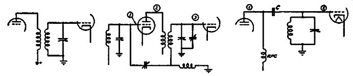
Resonance in tuned circuits is obtained either by series tuning or parallel tuning. The former type of circuit is known as a series resonant circuit and it is characteristic of series resonant circuits that maximum current flows during the state of resonance and, since the impedance of the circuit is then a minimum, it is possible to accomplish two things; one of these is to utilize the low impedance as a short-circuiting path at the resonant frequency, or as a trap circuit, and the other is to employ the device so that the maximum current is allowed to flow through the de sired circuit at resonance. These two applications, though identical in basic design, differ in circuit arrangement, and are shown ...

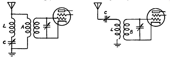
FIGs. 4-1(a) (left), 4-1(b) (right). The wave trap, L and C in the circuit at the left, by-passes the signal at the resonant frequency and thus rejects it. In the circuit at the right the signal at the resonant frequency is passed on to the secondary.

... in Figs. 4-1 (a) and 4-1 (b). In Fig. 4-1 (a), the wave trap LC is the series circuit used as a short-circuiting impedance at resonance. It is shunted across the antenna coil A and its purpose is to by-pass the current at the resonant frequency. If we assume that the function of this circuit is to by-pass an interfering signal of, say, 465 khz, tuning this circuit to 465 khz will prevent the development of a signal at this frequency across the antenna coil; consequently, there will be no signal voltage at this frequency applied to the r-f amplifier tube. The impedance of the circuit being limited solely by the circuit resistance, is consequently very low; much lower than that of the antenna coil A. The lower the resistance of the circuit, the less its impedance at resonance and the greater its selectivity. The greater the selectivity of this circuit, the less its effect upon signals higher or lower than the resonant frequency. In other words, its trap action becomes sharper as the selectivity is increased.

Another application of the same principle, but employed differently, is shown in Fig. 4-l(b). Land C now constitute the tuned circuit in the antenna system. The impedance is a mini mum at resonance, consequently the maximum amount of current flows through the system. Coil B, being coupled to L, receives the maximum amount of energy. In Fig. 4-1 (a), the resonant circuit is used to trap out or reject a certain signal, whereas in Fig. 4-1 (b) the same principle is employed to accept the desired signal.

Still another practical application of series circuits is the scratch filter used in connection with phonograph pickups and audio amplifiers. The series-resonant circuit, tuned to the approximate frequency of the scratch, is connected across the pickup and its purpose is to by-pass or short-circuit the balance of the system at this noise frequency by offering a low impedance path.

The Parallel-Resonant Circuit

The parallel-resonant circuit finds far more extensive application in radio receivers than the series-resonant circuit. This condition is not due to any difference in the operating efficiency of the two circuits, but rather to the fact that the arrangement of the elements of the parallel circuit is such that the coil presents a ready path for the application of operating voltages to the elements of the respective tubes. Perhaps the most important reason for the greater use of the parallel tuned circuit is that it offers a high impedance at resonance, while the impedance of series tuned circuits is very low at resonance. Since it is necessary to provide a high-impedance load in order to obtain any degree of amplification from a vacuum tube, the reason for the more frequent occurrence of the parallel-resonant circuit is at once apparent.

Series and parallel tuned circuits find a number of different applications. In this section, we are primarily concerned with their applications at frequencies within the r-f and i-f bands wherein they serve to select desired signals and to exclude interfering signals. While the parallel-resonant circuit is occasionally employed as the sole coupling medium between r-f and i-f amplifying tubes, by far its widest application is in single-tuned and double-tuned transformers in which the primary and secondary circuits are inductively coupled.

The Simple Tuned Transformer

The simple tuned transformer shown in Fig. 4-2, consisting of a single tuned secondary circuit coupled to an untuned primary circuit, is productive of a resonance curve which has but a single ...

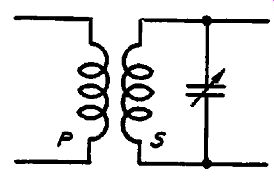
Fig. 4-2. A simple two-winding transformer. The primary is untuned, while the secondary is tuned by means of the shunt condenser.

... peak at resonance. With respect to the width of the curve, the resonance curve for a complete transformer is somewhat wider than for the transformer secondary alone-taken with the primary absent. The presence of the primary-untuned though it may be-has the effect of introducing some resistance into the secondary winding. Maximum signal transfer from the primary to the secondary winding occurs when optimum coupling exists.

Increasing the coupling beyond this point will reduce the signal transfer somewhat and will tend to broaden the resonance curve.

Reducing the coupling below the optimum point will likewise re duce the signal transfer and make the curve narrower.

As far as coupling is concerned, what is said about the simple tuned circuit transformer is true about all other types- that is, with respect to optimum coupling. The shape of the resonance curve may change with other types of transformers, but for each there is an optimum adjustment of coupling, sometimes expressed in terms of the coefficient of coupling which provides maximum transfer of energy. At this time we wish to add that, with the exception of those transformers which are provided with means for changing the coupling, you who may have occasion to service finished receivers should not change the coupling in the transformers. The desired condition will be obtained by correct alignment. Of far greater importance is that you should know the type of resonance curve to be attained, in accordance with the type of transformer involved. Let us now consider the most popular type of transformer used in modern radio receivers: the double-tuned transformer.

The Double-Tuned Transformer

The double-tuned, inductively-coupled transformer is illustrated in Fig. 4-3. The basic description of such a transformer is one in which two separate circuits, coupled to each other, are ...

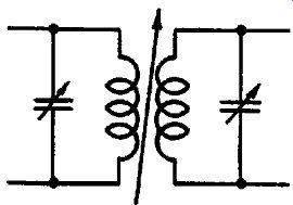
FIG. 4-3. A conventional i-f transformer with both primary and secondary windings tuned. The arrow between the windings indicates that the coupling be tween the windings can be varied.

... tuned to the same frequency. Some variations of this condition will be found in practice as outlined later, but the basic condition is as has been stated. In this transformer both the primary and secondary are parallel resonant circuits. This is common practice as far as receiver application is concerned, but what will be said applies equally to transformers in which either or both circuits are of the series-resonant type, and whose inductances are inductively coupled. What happens in this type of unit under two conditions--first, the effect of coupling and second, the effect of incorrect tuning?

What can we expect when the coupling is varied? In accordance with the function of coupling and from what has been said in connection with the simple single-tuned transformer, it is more or less obvious that the overall resonance curve is going to depend on the coupling. In order that the effect of coupling be illustrated in the most practical manner, a conventional i-f transformer of the commercial variety used in a modern superheterodyne receiver was arranged to simulate working conditions and in such manner that the coupling could be changed at will. The unit was connected into an oscillograph circuit so that oscillograms of the overall resonance curve could be taken. The constant-voltage input to the transformer was obtained from a frequency-modulated oscillator. The two windings were tuned accurately to the same frequency, with minimum coupling between the windings, so that there would be no reaction between the windings and accurate tuning would be possible (For a complete description of how such curves are made with the cathode-ray oscillograph, see Rider's The Cathode-Ray Tube At Work.)

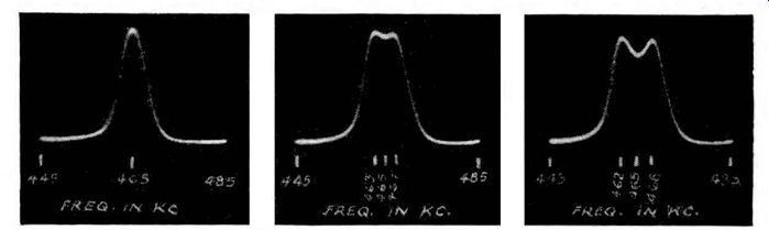
The amplitude of the response curve for each condition of coupling is representative of the actual performance of the unit under the conditions named. The results are shown in the series of nine oscillograms given in Fig. 4-4 and are for increasing values of coupling, beginning with minimum coupling, which would result in the transfer of just sufficient energy so that a resonance curve could be obtained.

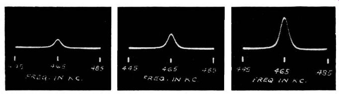
Figs. 4-4(a), 4-4(b), 4-4(c), left to right. As the coupling between the two windings is increased, more and more signal is passed, as can be seen from the increasing height of the signal across the secondary.

The effect of increasing coupling is evident in Figs. 4-4(a), 4-4(b) , 4-4(c) and 4-4(d). As you can see, increasing the coupling from the minimum point results in an increase in signal transfer until a critical point is reached where there is no further increase in the amplitude of the response curve, but there is a slight broadening of the peak. Fig. 4-4(d) illustrates the curve with the slightly broadened peak. During this time, there has been no change in the tuning or in the magnitude of the signal voltage fed into the test circuit. The frequency-modulated oscillator supplies a signal voltage which varies from about 445 khz to 485 khz twenty-five times per second and is constant in voltage over this range. The resonant frequency of the transformer is 465 khz.

Up to this time the effect of an increase in coupling is to in crease the energy transfer. Neglecting the very slight amount of interaction between the primary and secondary, as indicated by the slightly broadened peak, we can say that critical coupling exists. A slight increase in coupling, with everything else un changed, develops the curve shown in Fig. 4-4(e). Note that the amplitude of the curve does not change, but the shape of the …

Figs. 4-4(d), 4-4(e), 4-4(f), left to right. As the coupling is increased further, an optimum value is reached in Fig. 4-4(e). A further increase in coupling results in the development of a peak on each side of the resonant frequency.

... curve is changed in that two distinct peaks have been produced with a slight dip in the center. Also that the band width has increased at the top of the curve, as well as at the base. Note that the dip occurs at the point which was originally the peak and that one peak now occurs below the resonant frequency and another peak above the resonant frequency. A still further in~ crease in coupling develops the curve shown in Fig. 4-4(f), which illustrates an accentuation of the condition shown in Fig. 4-4(e). The dip is more pronounced and there is a slight decrease in the overall amplitude of the resonance curve. Also, the frequency band pass is increased as indicated by the increased separation between the two peaks.

The interaction between the primary and secondary windings, as a result of the higher degree of coupling, is manifesting itself.

Coupling which produces a double-peaked, or doubled-humped, resonance curve is known as close coupling. Naturally, there are various degrees of close coupling, as is evident in Figs. 4-4(e) and 4-4(f) and more to follow. The following is a brief explanation of why the resonance curve appears as shown.

For coupling in excess of the critical or optimum amount, the presence of the secondary winding reduces the current through the primary at the resonant frequency. Since the current in the secondary circuit conforms, to a major extent, to the primary current variations, a dip at the resonant frequency occurs. The greater this current, the greater is the dip. At frequencies above and below resonance, the effect of the secondary is to increase…

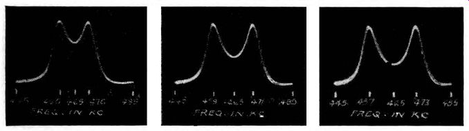
Figs. 4-4(g), 4-4(h), 4-4(i), left to right. As the coupling is increased still further, the frequency at which the peaks occur departs further from the resonant frequency and the dip between peaks increases.

... the primary current to values greater than those when the secondary is absent. The closer the coupling, the further apart the two peaks and the greater the dip at the resonant frequency-simultaneous with a gradual reduction of the amplitude of the curve.

This is shown in Figs. 4-4(g), 4-4(h) and 4-4(i), where Fig. 4-4(i) is the maximum coupling possible with the i-f transformer used in the test.

When external influences such as regeneration are absent, the resonance curve is quite symmetrical. By this is meant that the variations in the curve are essentially the same both sides of the resonant frequency and the amplitude of the two peaks is the same.

Let us now analyze the curves of Figs. 4-4 (a) to 4-4 ( i) and see what can be learned concerning the resonance curves of such double-tuned transformers. First, it is evident that such a trans former is capable of providing a single-peaked or a double-peaked resonance curve. Whichever is developed depends upon the degree of coupling. Second, that unless external and undesired influences are present, the curve should be symmetrical. This is of value when the resonance curve is established by any one of the numerous means available, as will be stated later. Third, because of the range of resonance curves possible with such a unit, it is possible to increase the band of frequencies passed by the device provided that the coupling is variable. However, in the event that the coupling is fixed, then the optimum setting is that which can be secured solely by correct tuning. If the design of the transformer is such that the curve of Fig. 4-4(d) is the correct figure, then the correct tuning and correct conditions will develop such a curve.

Correct tuning can be stated as being that which provides the maximum amplitude for the resonance curve, consistent with the proper frequency band pass. Information concerning the frequency band pass is given under the heading "Selectivity Requirements," later in the section.

What happens if the two windings are not resonated to the same frequency? The major effect is that the two curves are not ...

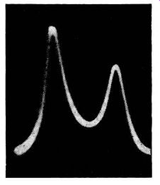
Fig. 4-5. Two peaks of different height are obtained in a closely coupled transformer when the primary and secondary windings are not tuned to the same frequency.

... of like amplitude. If the frequency of resonance in the primary circuit does not differ very greatly from the resonant frequency of the secondary circuit, then the two peaks will not be far apart; but if these two resonant frequencies differ widely, then the two peaks will be far apart and of unequal amplitude. Another effect is that the dip does not take place at either resonant frequency, but some place between-at least not midway between the peaks, as is the case when both primary and secondary circuits are tuned to the same frequency. Furthermore, the two peaks do not occur at the two resonant frequencies of the primary and secondary respectively. An example of an asymmetrical curve, or one with unequal amplitudes for the peaks, due to incorrect tuning, is shown in Fig. 4-5.

Selectivity Requirements

An understanding of the selectivity requirements and how these are related to fidelity of reception is highly desirable, because it establishes the type of resonance curve which should be developed and the advantage of one type of curve over another. Sup pose we consider the frequency composition of a 1000 -khz carrier, which is modulated with a 1000-cycle tone. Such a modulated wave consists of three frequencies-the 1000-khz carrier, the 1001 -khz upper side band and the 999 -khz lower sideband. This is ...

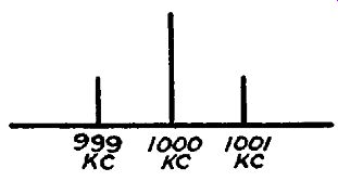
Fig. 4-6. When a 1000 -khz carrier is modulated by a 1000-cycle note, then the frequencies of the two sidebands will be 999 khz and 1001 khz.

... shown graphically in Fig. 4-6. If this same carrier is modulated by a 30-cycle tone, the frequencies in the wave are the carrier of 1000 khz, the upper sideband of 1000 khz + 30 cycles and the lower sideband of 1000 khz - 30 cycles. If the modulating frequency is 10,000 cycles, then the three frequencies are 1000 khz, 1010 khz and 990 khz. In actual voice transmission, the highest frequency used for modulation by the majority of broadcast stations is 5000 cycles, though a few high-fidelity transmitters use about 7500 cycles, or slightly higher.

In these examples we assume a constant tone for modulation.

If complex tones are used so that 30 to 5000 cycles is the band of modulating frequencies, then the upper and lower sidebands are limited by the highest modulating frequency. The carrier frequency remains as before, 1000 khz.

Now, an essential characteristic of a receiver is to pass the modulated carrier without suppression of the modulating frequencies. This means that those parts of the receiver which are required to pass the modulated carrier should be equally responsive to the sidebands as well as to the carrier. In order for this to be realized, the ideal response curve required for the various tuned circuits should be a square-topped curve with vertical sides.

The width of the top should be the full width of what is classified as the normal sidebands for normal broadcast transmission. . . . With 5000-cycle modulation this is 10 khz, or 5 khz each side of the carrier frequency. This is illustrated in Fig. 4-7. If the modulating frequency limit is 10,000 cycles, then each sideband is 10 khz wide and the total band width must be 20 khz.

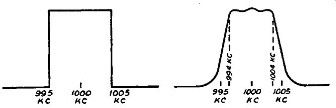
Figs. 4-7 (left), 4-8 (right). The ideal square-topped response for receiving signals which contain frequencies extending 5 khz on either side of the carrier. In practice, the response shown at the right approaches the ideal characteristic.

Up to the present time, square-top resonance curves have been impossible to attain, but an approach to this ideal has been reached. For example, the curves of Figs. 4-4 ( e) and 4-4 { f) show a fairly flat top. If you compare Figs. 4-4(d) and 4-4(e), you will note that while the amplitude or the response of both is substantially the same at the carrier frequency, which in this case is assumed to be the resonant frequency, the response 3 khz each side of the carrier is greater with the adjustment indicated by Fig. 4-4(e) than with the adjustment indicated in Fig. 4-4(d). In turn, the adjustment indicated in Fig. 4-4(f) shows greater response at about 5 khz each side of the carrier than either Figs. 4-4(d) or 4-4(e). At the same time, Fig. 4-4(f) shows less response at the carrier frequency than either of the other two oscillograms.

In the modern high-fidelity receiver, even a closer approach to the ideal is attained by developing a curve, such as that shown in Figs. 4-4(f) or 4-4(g), in the i-f system and depending upon r-f selectivity, which is most responsive to the carrier, as shown in Fig. 4-4 ( d), to fill in the dip between the two outside peaks.

The curve developed as a result of the combination of the response characteristics of the i-f amplifier, with a resonance curve such as that shown in Figs. 4-4 (g) and 4-4 (d), is shown in Fig. 4-8. The variation in amplitude between the peaks is not sufficient to cause any complications. At the same time, the proper band pass is obtained and the sides of the curve are a close approach to the straight lines of Fig. 4-7. The flat top of Fig. 4-7 is simulated by the top of the curve of Fig. 4-8.

Variable Selectivity Circuits

The effect of a very sharply tuned amplifier, which has a characteristic similar to that of Fig. 4-4 ( d), is to attenuate the outer sidebands and hence to attenuate the higher audio frequencies, which are contained in these sidebands. Thus, excessive selectivity results in reduced high-frequency (audio) response. It is for this reason that the intermediate-frequency amplifiers of al most all the high-fidelity receivers on the market incorporate some arrangement for broadening the response of the amplifiers so that the higher audio frequencies will not be lost. If you examine the modern receiver you will find that many systems are in use for accomplishing this result and also that they all depend upon the fact that the frequency response of a transformer becomes broader as the coupling is increased.

In the foregoing discussion we have considered the characteristics of coupling devices in which tuned circuits are involved and their general applications in r-f, mixer and i-f stages. Now let use see how these and other coupling devices are employed in specific receivers.

Antenna Coupling Circuits

In commercial radio receivers, a large variety of devices have been employed to couple the antenna circuit to the input grid of the first tube. Fig. 4-9 shows one of the earlier coupling devices used for this purpose. The signal voltage from the antenna is applied across a simple potentiometer which serves as a volume control by enabling the signal voltage applied to the first r-f tube grid to be varied.

In Fig. 4-10, the antenna coupling device is also a volume control which serves to vary the cathode bias on the first r-f tube and, at maximum bias setting, to ground the antenna so that the ...

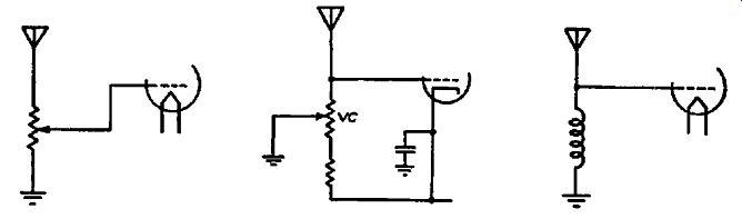
Figs. 4-9, 4-10, 4-11, left to right. Three methods for feeding the signal from the antenna to the grid of the first r-f tube are shown in the figures. No provision for tuning to the frequency of the signal is made in any of these circuits.

... signal voltage applied to the r-f tube grid is a minimum when the cathode bias is maximum. This affords a wider range of control than is possible with the simpler system shown in Fig. 4-9. This type of control has been used in a very large number of small receivers which do not employ automatic volume control.

In Fig. 4-11, the coupling device from the antenna to the r-f tube is an r-f choke, which is designed so as to have a substantially uniform impedance over the broadcast band. In the three coupling circuits just described, there is no step-up in signal volt age from the input terminals of the receiver to the first r-f grid and also, since the input circuit is untuned, these coupling circuits have no ability to discriminate between signals of different frequencies and are consequently not selective.

Most present-day receivers employ single-tuned transformers to couple the antenna circuit to the first tube. In Fig. 4-12, this type of input circuit is shown in its simplest form. The primary coil is usually designed to resonate at a frequency below that of the band over which it is to operate, so that its impedance is high at the low-frequency end of the band and low at the high frequency end of the band. The secondary circuit is tuned to resonance with the signal frequency. When this is done, the signal voltage developed across the primary coil is amplified and applied to the grid of the first tube. The signal amplification, due to the transformer, varies in different receivers, ranging from about 2 to 10 in home broadcast receivers and from 10 to 50 in automobile receivers.

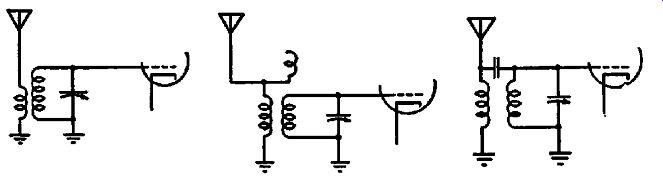
Figs. 4-12, left, 4-13, and 4-14. Three methods for coupling the signal from the antenna to the grid of the first r-f tube. Each of these circuits is tuned to the frequency of the desired signal by means of a. variable condenser.

With the simple design shown in Fig. 4-12, the antenna I transformer may provide less signal amplification at the high frequency end of the band than it does at the low-frequency end.

This is usually due to the design of the primary coil, the impedance of which is higher at the low-frequency end of the band. To increase the gain at high frequencies, a small amount of capacity coupling from the antenna coil to the secondary coil is often added, as shown in Fig. 4-13. Note that this is capacitive coupling and not inductive coupling, even though a few turns in the form of a coil is used, its inductance is practically zero. In Fig. 4-14, a small condenser is shown, joining the primary and secondary windings. This condenser is employed for the same purpose as the small coil shown in Fig. 4-13.

Image Suppression Circuits

In superheterodyne receivers, a high degree of selectivity is desirable in the circuits preceding the mixer tube. In the formation of the intermediate frequency, the local oscillator in such receivers beats with all signals which are present in the mixer input circuit. If undesired signals of certain frequencies are present, it is possible that they, too, may appear in the mixer plate circuit and be amplified by the i-f amplifier along with the desired signal. This causes interference, chirps and other troubles which cause objectionable reception.

One of the principal causes of such troubles is image-frequency interference. In receivers which employ an oscillator frequency higher than the signal frequency, the image frequency is equal to the signal frequency plus twice the intermediate frequency. In receivers which employ an oscillator frequency lower than the signal frequency, the image frequency is equal to the signal frequency minus twice the intermediate frequency. In the first case, if the receiver is tuned to 1000 khz and the intermediate frequency is 180 khz, the oscillator frequency is 1180 khz. This 1180 -khz oscillator frequency will beat with any 1360 -khz signal present in the mixer input circuit to produce an intermediate frequency of 180 khz in the same manner as the 180 -khz i-f signal is produced from a 1000 -khz signal to which the receiver is tuned. If the signal volt age of the 1360 -khz signal at the mixer input were the same as that of the desired 1000 -khz signal, they would be of equal strength and frequency at the input to the i-f amplifier. The same situation ...

Figs. 4-15 (left), 4-16 (right). Two circuits for obtaining r-f selectivity and minimizing image response. Their operation is described in the text.

... exists in receivers in which the oscillator frequency is lower than that of the signal, but in this case, the interfering image frequency, under the conditions previously specified, would result from the presence in the mixer input circuit of a 640 -khz signal where the receiver is tuned to 1000 khz.

To render this type of inter£ ere nee negligible, additional tuned circuits between the antenna and the mixer input grid are some times used. Often one or more tuned r-f stages are employed, but in modern receivers which are not so equipped, a high inter mediate frequency is employed. If the intermediate frequency, for instance, is 465 khz instead of 180 khz, the image frequency will differ by 930 khz from the signal frequency. This wide frequency separation is often sufficient to render special image suppression circuits unnecessary in most localities, even when only a single tuned circuit precedes the mixer.

Examples of image suppression circuits are shown in Figs. 4-15 and 4-16. As you will note in Fig. 4-15, the antenna coil is inductively coupled to an intermediate tuned circuit which, in turn, is similarly coupled to the mixer input tuned circuit. If a signal is fed to the antenna coil, the signal amplification due to trans former action is maximum at point !8 when the intermediate circuit is turned to resonance with the incoming signal. Since there is some loss in coupling, the signal strength at point S will not be as great as at point 2. However, the selectivity will be improved, since the intermediate tuned circuit acts as a filter.

In Fig. 4-16, a special circuit is shown which is used for image rejection in many early Atwater Kent superheterodynes, such as the 72, 74 and 76 series. This is called the double spot system.

Since the intermediate frequency. employed is 130 khz, the image frequency occurs at 260 khz above the signal frequency. The image-suppression circuit is adjusted to resonate at a frequency 260 khz higher than that of the r-f tuning system. The double spot trimmer is adjusted by feeding a 1500 -khz signal to the input terminals of the receiver and tuning the receiver to 1240 khz. The double-spot trimmer is then adjusted for minimum receiver output. It is assumed that the r-f system has previously been aligned in the usual manner at 1500 khz.

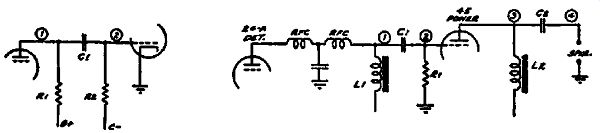
Radio-Frequency Coupling Devices

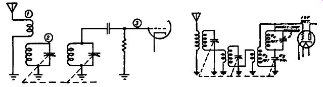
Typical r-f coupling systems used in radio receivers are shown in Fig. 4-17. The r-f transformer illustrated in Fig. 4-17 (a) rep resents a type which is in general use in modern radio receivers.

Figs. 4-17(a), 4-17(b), 4-17(c), left to right. Typical r-f coupling systems used to transfer the signal from the plate of an r-f tube to the grid of the succeeding tube.

Such a transformer is used to couple the plate of an r-f amplifying tube to the grid of the following tube. For efficient operation the design of any coupling transformer depends upon the type of tubes which are being coupled. In modern receivers, r-f amplifying tubes are of the pentode type which have a high plate resistance and require a high-impedance plate load for maximum signal amplification. Consequently, the primary of such r-f transformers, which forms the plate load, is designed to have a high impedance to frequencies over its operating range. In this way, the amplifying properties of the tube are most efficiently utilized.

In such r-f transformers, little or no gain is obtained from the transformer action itself, since both the secondary and the primary circuits have a high impedance to the signal frequencies.

We can obtain amplification from transformers only when the impedance of the secondary and its load is higher than that of the primary circuit. With triodes, which formerly were widely used in r-f amplifiers, the plate load, or transformer primary, is of low impedance since the plate resistance of triodes is much lower than that of pentodes. The tuned secondary, however, has a much higher impedance than that of the primary and consequently the signal is amplified by such coupling transformers. The signal amplification obtained in this manner by the transformer is often greater than that obtained from the triode, though the combined gain from both sources is less than is obtained from pentodes.

In a typical receiver employing triodes in the r-f section, such as the Majestic 90 shown in Fig. 4-17(b), the measured gain of each r-f stage was found to be 10. The gain from point 1, the control grid, to point 2, the plate of the r-f triode, was only 2, while from point 2 to point 3 the measured gain was found to be 5. Since the stage gain is the product of the transformer gain and the tube gain, the total gain for the single stage at one frequency is 10. In modern pentode r-f amplifiers, there is usually no gain in the r-f transformer but the gain due to the tube ranges from 10 to 40. A complete table of gain-per-stage values is shown in Section 9.

Fig. 4-17(c) shows the form of coupling used in an r-f stage of the Midwest Model 9-31 receiver. As shown, the plate load for the r-f tube is an r-f choke and the coupling to the grid of the following tube is effected by means of the coupling condenser C. There is no signal amplification in this form of coupling, the signal level at the plate of the r-f tube point t, being the same as that at the control grid of the following tube, point f. The signal gain is obtained entirely by the r-f tube and its plate load.

I-F Systems

We have already discussed the characteristics of coupled circuits used in i-f systems and the effect of various degrees of coupling upon the performance of the coupling unit. From the signal tracing standpoint, we are also interested in the gain or loss which results from the use of various types of i-f coupling methods. In practically all commercial radio receivers, transformers are used for coupling in i-f stages. Also, we find that the primary and secondary windings are tuned to the intermediate frequency.

This means that both windings normally present a high impedance to the signal frequency and consequently, as pointed out in the discussion of r-f transformers, we can expect little or no gain in the i-f transformer itself. A decrease in stage gain will result from any factors which lower the impedance of primary and secondary circuits of such transformers. Such a condition may result not only from misalignment, since the impedance is greatest at resonance, but also may occur due to moisture absorption, de crease in coupling due to shifting of the position of one coil with respect to the other, as well as from troubles arising in other components of the i-f stage.

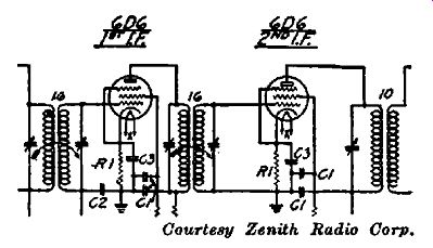
FIG. 4-18. The selectivity of the i-f amplifier is con trolled by varying the coupling between the primary and secondary windings in the first two i-f transformers. Zenith Radio Corp.

A direct application of the principles previously discussed is found in the Zenith Stratosphere. That part of the receiver which concerns us is shown schematically in Fig. 4-18. As indicated by the conventional arrow, the coupling in the first and second i-f transformers is continuously variable. This receiver is representative of that type which uses a mechanical variation of the coupling in a two-winding transformer to accomplish a continuous variation of the selectivity. It is interesting to note that only the first two i-f transformers are so controlled, the response of the third i-f transformer being sufficiently broad so that the sidebands are not appreciably attenuated.

The Wells-Gardner Model

ODM is typical of the class of receivers which uses a switching arrangement to obtain various degrees of coupling in the i-f amplifier. Referring to the partial schematic shown in Fig. 4-19, you can see that a third winding…

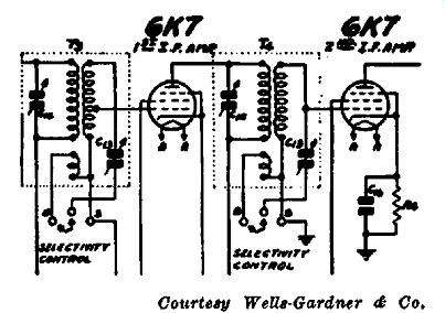
Fig. 4-19. A variable selectivity circuit employing an auxiliary winding to control the coupling.

… is included in the first and second i-f transformers. The primary and secondary are loosely coupled, while the auxiliary winding is closely coupled to the primary winding. The required close degree of coupling is obtained by winding the third coil underneath the primary. By means of the selectivity control switch, this third winding can be put into or out of the circuits. Two values of coupling are provided. With the switch in the "broad" position, the third winding is part of the secondary tuned circuit and the effect is to produce a large value of coupling between primary and secondary. With the switch in the "sharp" position, the third winding is out of the circuit and the resultant coupling is loose.

The result is a sharp selectivity characteristic. The coupling in the second i-f transformer is controlled in the same way and the two selectivity control switches are ganged to form the overall selectivity control. A general idea of what represents a "sharp" selectivity characteristic is shown in Fig. 4-4 ( d) and Fig. 4-4 (f) illustrates in a general way, a "broad" characteristic.

A slightly different variation of the same principle is used in the Fairbanks-Morse 100. Reference to Fig. 4-20 shows that the secondary is composed of three sections--L3, L4, and L5. The primary is composed of L1 and L3. L1 and Lt are loosely coupled to each other and constitute the major portion of the primary and secondary inductances respectively. LS and L4 are tightly coupled, while the coupling between L5 and the primary is loose. With the switch in the broad position, L5 is out of the circuit and the secondary winding consists of Lt and L4. Since L4 is closely coupled to L3, the coupling between the secondary…

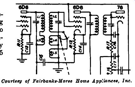
Fig. 4-20. A variable selectivity circuit employing a transformer with two auxiliary windings. Coupling is controlled by switching either L4 or L5 into the circuit.

…and primary windings is sufficiently great so that a broad response is obtained. With the switch in the "sharp" position, the closely coupled L4 is replaced by L5, which has the same inductance but is loosely coupled. Thus, in this position the overall coupling between primary and secondary is low and hence the frequency response is sharp. The alignment is not disturbed when changing from the sharp to the broad selectivity position.

Up to the present point we have limited our discussion to i-f transformers wherein selectivity is a function of the coupling between two tuned circuits. A variable-selectivity type of three winding transformer in common use is shown in Fig. 4-21 ; this is a partial schematic of the Stromberg-Carlson Model 70. Note that the first and second i-f transformers consist of three tuned circuits. Transformers of this type operate in the following manner: The primary and secondary windings are loosely coupled, while the third or tertiary winding is closely coupled to the secondary winding. When the resistance in series with the tertiary winding is greatest, the tertiary tuned circuit draws practically no current and consequently there is practically no reaction be tween it and the other windings. Thus the transformer operates as an ordinary loosely coupled two-winding transformer to pro vide normal, sharp selectivity and reduced band-width. In the maximum selectivity position, a switch operated by the selectivity or fidelity control, opens the tertiary tuned circuits completely.

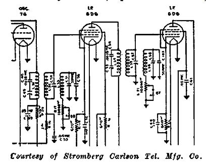
Fig. 4-21. In this circuit the selectivity is controlled by varying the series resistance in the tertiary tuned circuits.

Now let us see what takes place when the third winding is in the circuit and the resistance in the tertiary tuned circuit is decreased.

This circuit, being tuned to the i-f peak, acts as a load across the secondary winding, abstracts energy there from, and produces a broadened response. This effect is most pronounced, of course, when all resistance is out of the circuit, for then a maximum current flows in the tertiary circuit and there is a maximum broadening of the frequency response. This is the high-fidelity position and results in a selectivity characteristic similar to Figs. 4-4 ( e) or 4-4(f). The Philco 201 is another example of a receiver using three winding i-f transformers, with a variable resistance in series with the tertiary winding to control the selectivity and band-width. At this stage you may be interested in the manner in which the response characteristics of such three-winding transformers change during manipulation of the control.

The three oscillograms in Fig. 4-22 indicate how the form of the selectivity curve changes with the magnitude of the resistance in the tertiary tuned circuit. Fig. 4-22(a) is the response of an amplifier employing two transformers of this three-winding type and one closely coupled two-winding i-f transformer; this is for maximum selectivity or maximum resistance in the tertiary circuits. Fig. 4-22(b) is the response of the same i-f amplifier with an intermediate value of resistance in the tertiary circuits. Note how the selectivity is broadened as against the sharp response of Fig. 4-22 (a) . With no resistance in the tertiary circuits, the absorption of energy at the peak frequency results in the familiar dip and greatly increased band-width, as is shown in Fig. 4-22(c). An intermediate setting between Figs. 4-22(b) and 4-22(c) results in a fiat top.

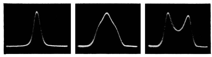
Figs. 4-22(a), 4-22(b), 4-22(c), left to right. The overall response of a three-winding transformer is shown for three different values of resistance in series with the tertiary circuit. Note the broadened response obtained as the resistance is decreased.

While on the subject of three-winding transformers, the function of the transformer used in the Atwater Kent Model 856, Fig. 4-23, is not to provide a control over the selectivity, but to make ...

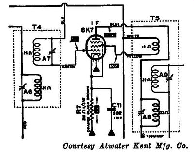
Fig. 4-23. The third winding feeds back a portion of the voltage from the plate to the screen circuit in the correct phase to prevent oscillation.

... possible increased gain in the i-f stage by stabilizing the amplifier. This, as can be seen from the schematic, is accomplished by using the third winding to feed back a portion of the voltage from the plate to the screen circuit in the correct phase to prevent any tendency toward oscillation.

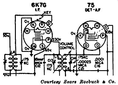
Fig. 4-24. The volume is controlled by varying the coupling between the primary and secondary windings. Sears Roebuck.

In the oscillograms shown in Fig. 4-4, we showed how the gain as well as the selectivity was dependent upon the degree of coupling. A practical example of such gain control is shown in Fig. 4-24. The volume control in this receiver is effected by varying mechanically the coupling between the primary and secondary of the last i-f transformer. It should be noted that there is no appreciable change in selectivity with this arrangement, since the coupling is at all times sufficiently loose so that there is negligible reaction between primary and secondary. This arrangement is used in several receivers made by Sears-Roebuck.

AUDIO-FREQUENCY COUPLING CIRCUITS

Types of coupling circuits used in a-f amplifiers may be divided into the following classes: (1) Resistance coupling; (2) Transformer coupling; (3) Choke coupling; (4) Direct coupling.

Practically every commercial radio receiver employs one or more of these types of coupling in the a-f amplifier section of the receiver, resistance and transformer coupling being used almost exclusively in all modern receivers. Choke coupling was rather widely used in earlier receivers, before the introduction of the tetrode and pentode, because the triodes then available required high plate current for efficient operation and this could not be obtained without using excessively high power-supply voltages to make up for the voltage drop which would necessarily occur when high resistance was placed in the plate circuit. The high plate resistance and low plate current of pentodes, tetrodes and high-mu triodes enable the use of high-resistance plate loads with satisfactory operation at normal power-supply voltages. Furthermore, the latter types of tubes are capable of providing far more signal amplification than is possible with earlier triodes.

In power output stages, transformer coupling is essential for efficient operation in modem receivers because this is the most satisfactory method of coupling the relatively high-impedance power tube plate circuit to the very low-impedance voice coil of the modern dynamic speaker.

Figs. 4-25 (left), 4-26 (right). Two circuits for coupling the signal from plate to grid. The circuits are described in the text.

In Fig. 4-25, a partial schematic of a typical resistance-capacity coupled amplifier stage is shown. The amplified audio signal voltage is developed across Rt and is measured at point 1, the amplifier tube plate. The coupling condenser, Ct, serves to transfer the a-f signal to the grid of the following tube and, at the same time, prevents the high d-c voltage present at the plate from being impressed on the control grid of the following tube. Except at very low audio frequencies, the reactance of the coupling con denser is sufficiently low so that the signal voltage appearing at point 2 is substantially the same as that at point 1.

Choke Coupling

In Fig. 26, the a-f system of the Radiola 44 is shown. The plate load of the type 24-A detector is a high-impedance a-t choke Lt, the inductance of which is approximately 300 henries.

A choke of such high impedance is necessary because the type 24-A tube has a high plate resistance and the plate load must always be much higher in impedance than the plate resistance of the tube with which it is used, if distortion is to be kept low.

In the output circuit, the plate load is actually the magnetic speaker, with which this set was designed to be used. The choke LS, acts merely as a path for the plate current of the type 45 tube. This is done because the high d-c plate current required by this tube might affect the operation of the speaker. The impedance of the L2 is high with respect to that of the speaker so that very little power is lost in the choke.

The signal level at point 2 will be substantially the same as that at point 1, since the impedance of the coupling condenser C1 is very low with respect to Rt, over most of the a-f range. In the output circuit, when a speaker is connected, the signal voltage at low audio frequencies will be somewhat lower at point 4 than at point 3. If C2 is open, there will be no signal at point 4 though the signal will be normal at point 3. If C2 is shorted, connecting the speaker will short-circuit the plate voltage. With the speaker disconnected, the signal level will be the same at points 3 and 4, but of course the d-c plate voltage will be present at point 4 as well as point 3.

Figs. 4-27, 4-28, 4-29, left to right. Three methods for obtaining inter stage coupling. The operation and signal distribution are described in the text.

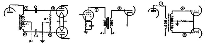
Push-pull operation is sometimes obtained by means of a tapped choke, as shown in Fig. 4-27, which represents the a-f system employed in the Stromberg 29 receiver. The plate voltage is fed to the a-f tube by means of a center-tapped choke Lt. The a-f voltage is developed across the entire choke, so the signal voltage at point 1 is normally the same as that at point 2, but these signal voltages are opposite in phase. The signal voltages at points 3 and 4 should likewise be equal.

Interstage Transformer Coupling

In the partial schematic diagram Fig. 4-28, the a-f transformer is used to couple the relatively low-impedance plate circuit of the amplifying triode to the high-impedance grid circuit of the fallowing tube. In Class A amplifiers, a signal voltage step-up from point 1 to point e of two or three-to-one is normal; therefore the signal level will be appreciably higher at point 2 than at point 1.

In push-pull input stages, such as that shown in Fig. 4-29, only one-half the total signal voltage across the a-f transformer secondary is applied to each grid. Consequently, the signal voltages at points 2 and 3 will normally be very little higher than at point 1.

In Class B input stages, a step-down ratio is required from the primary to the secondary winding so the signal voltage will normally be less at points 2 and 3 than at point 1. The signal distribution in Class A, driver, and Class B stages is discussed in Section 2 in the section on power amplifiers.

DIRECT COUPLING

As the name implies, a direct-coupled amplifier is one in which each stage is directly coupled to the preceding one, so that coupling condensers and transformers are eliminated. In practice, the grid of each stage is connected directly to the plate of the preceding tube. Because this places the grid at the same positive voltage as the plate, direct-coupled amplifiers employ various methods for providing each tube with the proper bias voltage.

The primary purpose of direct-coupled amplifiers is to enable the amplification of d-c voltage and signals of very low frequencies. This is not possible with the conventional amplifier which employs either coupling condensers or transformers, for at very low frequencies the coupling condenser blocks the passage of the signal. In a similar way, the action of the transformer depends upon the production by the signal of a rapidly varying flux. At low frequencies this rapid variation does not exist and hence the signal is not transferred efficiently from the plate to the grid of the succeeding stage.

In a direct-coupled amplifier, a direct link or coupling is used and this provides the same voltage amplification of the signal regardless of the frequency. In fact, the amplifier functions just as efficiently for the amplification of direct currents and voltages as it does for alternating voltages. The gain of a direct-coupled amplifier is independent of frequency from the lowest value up to fairly high frequencies. The upper-frequency limit, as in the case of a resistance-capacitance coupled amplifier, is reached when the shunting effect of the tube capacitances becomes sufficiently great so that the signal is by-passed around the load resistances.

A simple direct-coupled amplifier circuit employing two stages is shown in Fig. 4-30. Note that the customary blocking condenser or coupling transformer is not used and instead the plate ...

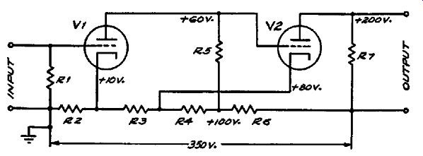
FIG. 4-30. A two-stage direct-coupled amplifier. The volt age distribution is indicated on the figure.

... of V1 is connected directly to the grid of V2. The necessity for a special biasing arrangement can now be seen. In the circuit shown, the voltage at the plate of V1 with no signal applied is equal to 60 volts. To obtain the correct bias voltage for V2, the cathode of V2 is returned to a point on the voltage divider which is 80 volts positive with respect to ground. As a result of this connection, the bias on the second tube--which is equal to the difference between the voltage at the grid and that at the cathode -is equal to -20 volts. The voltage supply to the plate of V1 is equal to 100 volts - 10 volts, or 90 volts. In the same way the plate voltage supply for the second tube is equal to 350 volts - 80 volts, or 270 volts.

To examine the method of signal amplification and transfer in a direct-coupled amplifier, let us assume that a positive voltage is applied to the input grid of V1. As a result of this positive voltage (or pulse), the plate current of V1 increases so that the volt age drop across R5 also increases. Since the voltage of points along the voltage divider remains essentially constant, it follows that the voltage at the plate of V1 decreases and the voltage at the grid of VS become more negative. This negative voltage at the grid of V2 causes the plate current of V2 to decrease. As a result, the voltage drop across R7 also decreases, so that the volt age at the plate of V2 increases above its normal value of +200 volts. In this way the original positive pulse of voltage applied to the input produces an amplified positive pulse of voltage across the output of the amplifier. Similarly, if a negative pulse of voltage were applied to the input of the amplifier, this same negative pulse would appear at the output but would of course be greatly amplified.

Insofar as the transfer of the signal is concerned, it is clear that the action which takes place is similar to that occurring in a conventional amplifier which employs coupling condensers. For this reason everything that has been said in connection with these amplifiers is applicable here so that a detailed discussion of signal tracing is not required.

Voltage Measurements

The importance of proper voltage measurements in a direct coupled amplifier cannot be over-emphasized. To avoid errors it is of the utmost importance that a high-resistance voltmeter be used, preferably one in which the resistance of the voltmeter is always at least twenty times as high in resistance as the resistance of that portion of the circuit being measured. If measurements are made with a voltmeter of low or even medium resistance, the operating conditions in the amplifier will be disturbed so greatly as to destroy the value of the measurements. Suppose, for instance, that the voltage at the plate of V1 is being measured with a low-resistance voltmeter. This will change the voltage at the grid of V2 because of the loading effect of the voltmeter and the direct coupling to the grid. In turn, the plate current of V2 will be changed and this will cause a change in the current flowing through R2 and R3. As a result, the normal division of voltages along the divider is completely changed. It should be noted that a somewhat similar effect occurs when a low-resistance voltmeter is used in a conventional amplifier. However, in the case of a direct-coupled amplifier, the error introduced by the voltmeter is amplified and reflected back so that the error is considerably greater than just the direct error produced by the voltmeter.