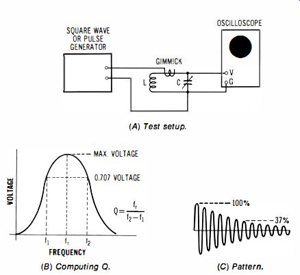
Fig. 6-1. Determination of bandwidth for LC circuit.
| Home | Audio mag. | Stereo Review mag. | High Fidelity mag. | AE/AA mag. |
6-1. To Measure the Bandwidth of an LC Circuit With a Ringing Test
Equipment: Square-wave or pulse generator that provides fast rise, coil, and capacitor (fixed or variable). Connections Required: Connect equipment as described in Fig. 6-1.
Procedure: Display the ringing waveform obtained with a chosen value of C, and count the number of peaks (cycles) in the ringing waveform from the 100 percent to the 37 percent amplitude point. Measure the ringing frequency.
Evaluation of Results: Multiply the number of cycles from the 100 percent to the 37 percent amplitude point by pi (3.14); this gives the approximate Q value of the LC circuit. Then, divide the ringing frequency by the Q value; this gives the approximate bandwidth of the LC circuit. As an illustration, suppose that the Q value of a coil is 50 and that the ringing frequency is 1 MHz. In turn, the bandwidth of the coil and its associated capacitance is approximately 20 kHz. Bandwidth is defined in this method as the number of cycles between the 0.707 voltage points on the frequency response curve. These 0.707 voltage points are also called the half-power points, or the -3 dB points.
NOTE 6-1 Resonant-Frequency Formulas
A damped sine wave such as shown in Fig. 6-1 has a frequency which is given approximately by the familiar resonant-frequency formula:
(B) Computing Q. (C) Pattern.
Fig. 6-1. Determination of bandwidth for LC circuit.
However, the exact ringing frequency is formulated:
We will find that when R has a small value, as in a color-subcarrier ringing-oscillator circuit. that the familiar resonant-frequency formula gives practically the same answer as the exact formula.
6-2. To Make a Ringing Test of an IF Transformer
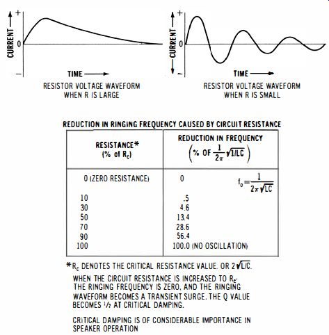
Fig. 6-2. Relation of natural frequency (ringing frequency) to the driven
resonant frequency, as in an amplifier load circuit.
*Re DENOTES THE CRITICAL RESISTANCE VALUE. OR 2{i]C. WHEN THE CIRCUIT RESISTANCE IS INCREASED TO Re· THE RINGING FREQUENCY IS ZERO. AND THE RINGING WAVEFORM BECOMES A TRANSIENT SURGE. THE Q VALUE BECOMES 'j, AT CRITICAL DAMPING. CRITICAL DAMPING IS OF CONSIDERABLE IMPORTANCE IN SPEAKER OPERATION
Equipment: Square-wave or pulse generator with fast rise.
Connections Required: Connect equipment as shown in Fig. 6-3.
Procedure: Display the ringing waveform, and adjust the trimmer capacitors (or slugs) for maximum pattern amplitude; well-defined zero-beat crossings will be observed at maximum amplitude.
Evaluation of Results: In general, this is considered to be a comparative test, to weed out defective transformers. However, a few of the pattern characteristics are of interest. An overcoupled if transformer has two resonant frequencies (two hump frequencies) which result from the mutual inductance between the two windings. These hump frequencies beat together to form the ringing pattern. If we call these ringing frequencies f1 and f2, the beat (envelope) frequency will be f2 – f1' The center frequency of the if transformer, such as 456 kHz, 4.5 MHz, or 10.7 MHz, is equal to the ringing frequency, or to (f1 + f2)/2.
NOTE 6-2 Adjustment of Primary and Secondary Frequencies
If the primary and secondary windings are not tuned to the same frequency in the procedure of 6-2, the ringing pattern will display peaks
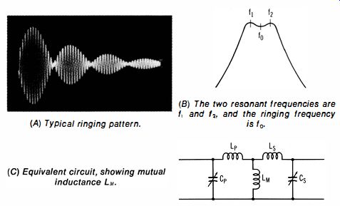
Fig. 6-3. Ringing test of an if transformer.
(A) Typical ringing pattern. (B) The two resonant frequencies are f1 and f2' and the ringing frequency and valleys but will not show any zero (crossover) points. As the primary and secondary frequencies are adjusted more nearly equal, the valleys in the waveform approach the zero level . At widely different primary and secondary frequencies, the higher frequency may appear merely as a "ripple" along the lower frequency.
6-3_ To Measure Percentage of Amplitude Modulation
Equipment: An am signal generator or other source of amplitude-modulated signal. Audio oscillator (if signal generator does not have audio output). Trapezoidal method requires an rf pickup loop and an RC coupling circuit, as shown in Fig. 6-4.
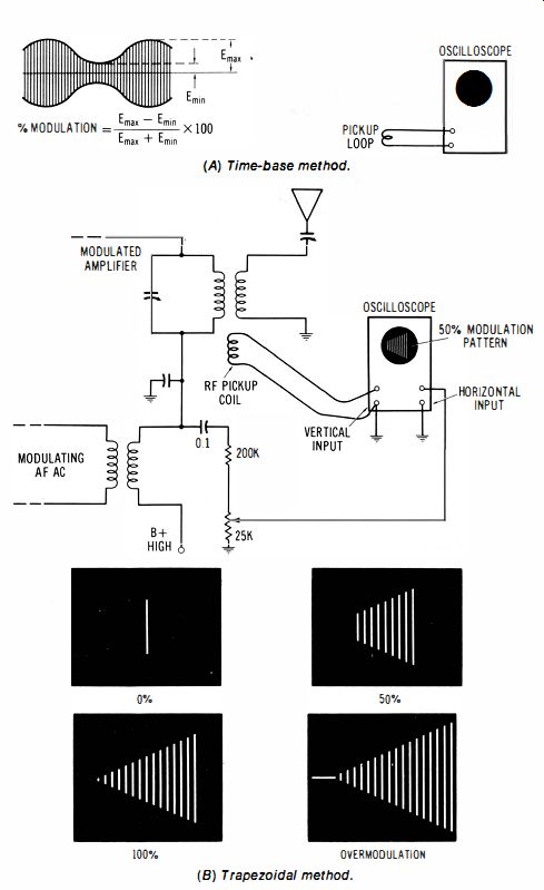
Fig. 6-4. Measurement of percentage amplitude. (A) Time-base method. (B) Trapezoidal
method.
Connections Required: When the time-base display is used, connect the source of the am signal directly to the vertical input channel of the scope. When the trapezoidal method is used, connect the pickup loop to the vertical-input channel of the scope, and connect the RC coupling circuit from the modulating voltage source to the horizontal-input channel of the scope.
Procedure: In the time-base method, observe the maximum and minimum peak voltages in the pattern. When the trapezoidal display is used , adjust the pickup coil orientation and the potentiometer for a trapezoidal pattern with proper layover; observe the relative vertical deflections at the ends of the trapezoidal pattern.
Evaluation of Results: Percentage of amplitude modulation is calculated as noted in the diagram.
NOTE 6-3 Distorted Modulation Patterns
Amplitude-modulation patterns may show various types of distortion.
For example, the illustration in Fig. 6-5 exemplifies typical inherent distortion for an economy-type am generator. This is an example of non-symmetrical and nonsinusoidal modulation. Residual frequency modulation is also present in the carrier, as a result of direct modulation of the rf oscillator. When trapezoidal displays are used, am distortion shows up curvatures or other distortions in the top and bottom of the trapezoid; the ends of the pattern may also be displaced vertically with respect to each other. Nonsymmetrical modulation causes a "double image" display, due to poor layover of the forward and reverse images.
Fig. 6-5. Output signal from an economy-type am generator.
6-4. To Check the Operation of an Op-Amp Integrator
Equipment: Square-wave generator.
Connections Required: Connect output from square-wave generator to input of op-amp integrator. Connect output from integrator to vertical input channel of scope (Fig. 6-6). Procedure: Observe output waveform over the rated repetition rate for the op amp.
Evaluation of Results: A precise triangular waveform is normally displayed on the scope screen. The useful range of the exemplified configuration is from 1 to 10 kHz, approximately.
NOTE 6-4 Op-Amp Characteristics.
An operational amplifier (op amp) is a very high gain integrated-circuit amplifier that is ordinarily used with considerable negative feedback.
In turn, the op amp has very low distortion, high stability, and a voltage amplification that depends on the value of the feedback resistance or feedback impedance. An op amp has comparatively high input resistance (in the absence of feedback), and a low output resistance. When a large amount of negative feedback is used, as in the example of Fig. 6-4, the input impedance of the op amp becomes very low, and can be regarded as a virtual ground. Consequently, the effective input impedance of the configuration is equal to the series input resistance that is used, plus the internal resistance of the source. Note also that an op amp has two input terminals; the inverting input is designated (-), and the noninverting input is designated (+). In the example of Fig. 6-4, the noninverting input is grounded via the 39 K resistor at terminal 4, and the inverting input is driven via Z, (the series input resistor, or weighting resistor). The weighting resistor determines the output/ input voltage ratio, with all other things being equal.
Fig. 6-6. Checking the operation of an op-amp integrator.
(B) Normal operating waveforms. (C) Typical package.
6-5. To Check the Operation of an Op-Amp Differentiator
Equipment: Square-wave generator.
Connections Required: Connect test setup as shown in Fig. 6-7.
Procedure: Observe the output waveform from the differentiator.
Evaluation of Results: A very narrow pulse output is normally produced at each leading and trailing edge of the squarewave input. Note that the 51-ohm resistor Zr in series with the input capacitor is used to minimize noise interference in the output (the resistor limits the rf gain of the op amp).
NOTE 6-5 Ideal Differentiator Action
An op-amp differentiator provides an output which more nearly approximates a true mathematical derivative than does an RC differentiator.
An ideal differentiator would produce an output pulse with infinite amplitude and infinitesimal width. Similarly, an op-amp integrator produces an output waveform which approximates a true mathematical integral more nearly than does an RC integrator. In other words, RC differentiators and integrators provide exponential output waveforms (Fig. 6-8),
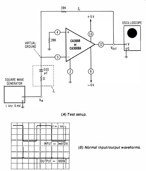
Fig. 6-7. Checking the operation of an op-amp differentiator. (A) Test setup.
(B) Normal input/output waveforms.
... whereas op-amp differentiators and integrators provide good approximations to straight vertical lines and straight-sided triangular waveforms.
(Op amps are used extensively in function generators and in analog computers.)?.
To Check the Operation of an Op-Amp Summer (Adder)
Equipment: Audio oscillator and square-wave generator.
Connections Required: Connect test setup as shown in Fig. 6-9.
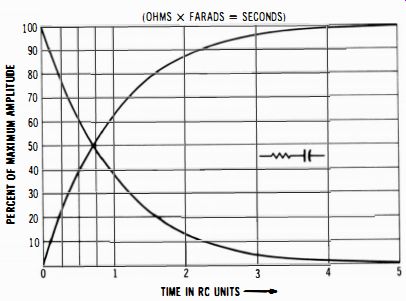
Fig. 6-8. RC differentiators and integrators produce exponential output waveforms.
Procedure: Adjust the audio oscillator output to a suitable level such as 90 mV p-p, and adjust square-wave generator output to a higher level, such as 180 mV p-p. Use different frequencies in the two input signals, such as 1 kHz and 100 Hz. Observe output waveform.
Evaluation of Results: As depicted in the diagram, an op-amp summer will normally produce the sum of the two input waveforms, at an amplified level : Observe that 1 K input (weighting) resistors are used in this example. Three, four, or more inputs, each with a 1 K input resistor, may be used, if desired, because terminal 3 of the op amp is a virtual ground, due to the large amount of negative feedback that is utilized.
NOTE 6-6 Subtraction by Op-Amp Summer
An op-amp summer will add dc voltages, if desired, in the same manner as it adds ac voltages. Note that a summer operates as a subtracter, if one of its inputs is reversed in polarity. Thus, +2 V added to +3 V equals +5 V; on the other hand, -2V added to +3V equals + 1V. Or, +2 V added to -3 V equals -1V. In the case of ac input voltages to a summer, the output waveform displays their sum when the two input waveforms are in phase with each other. On the other hand, the output waveform displays their difference when the two input waveforms are 180 degr. out of phase with each other.
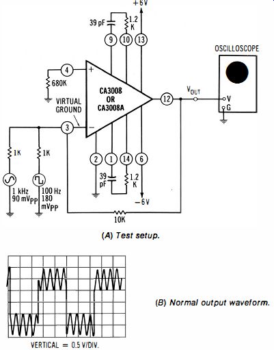
Fig. 6-9. Checking the operation of an op-amp summer (adder). (A) Test setup.
(B) Normal output waveform.
6-1. To Check the Operation of an Op-Amp Scaling Adder
Equipment: Audio oscillator and square-wave generator.
Connections Required: Connect test setup as shown in Fig.
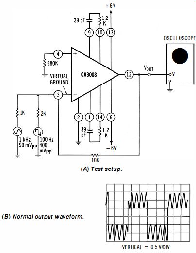
Fig. 6-10. Checking the operation of an op-amp scaling adder.
(A) Test setup. (B) Normal output waveform.
6-10. Procedure: Same as in 6-6.
Evaluation of Results: This op-amp adder employs a 1K input resistor for the sine-wave signal, and a 2 K input resistor for the square-wave signal. Practically, the gain for each input is calculated as the sum of the feedback and input resistances, divided by the input resistance. Thus, the gain is normally 11 times for the sine-wave signal, and 6 times for the square-wave signal. In turn, the output waveform normally appears as illustrated. The same test principles apply to more elaborate scaling adders that have more than two inputs.