Reviewed by Charles Hansen
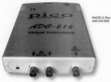
PHOTO 3: Pico
Pico ADC-216, $800 US, Pico Technologies Ltd., Broadway House, 149 151 St, Neots Rd., Hardwick, Cam bridge CB3 7QJ UK, (0) 1945 211716, picotech.com; US Distributor: Saelig Co., 1193 Mosely Rd., Victor, NY 14564, 716-425-3753, saelig.com.
The ADC-216 interface unit (Photo 3) is $25°W x 1.379"H x 7.125"D. The front panel has two BNC jacks for two-channel operation, and a third jack that serves as an external trigger input.
The box connects to the LPT1 printer port with a supplied data cable, and is powered by a 12V DC plug-in adapter.
An LED power indicator is located on the front panel (there is no power switch).
This LED also seems to function as a data acquisition indicator, based on its in-sync blinking with screen updates. You must power-up the box before you start the program or connect scope probes to a live signal. The ADC-216 is designed to use standard 1x or 10x scope probes, and has software scaling.
Software Included
The PicoScope software installation is simple and straightforward, and it needs only 2.3MB of free hard disk space. The PicoTHD program takes an additional 300KB. An uninstall program is also provided. Since Pico makes a number of other PC-based instruments, you must en able the ADC-216 during installation.
You also have the option of loading drivers for other operating environments.
You can even insert custom-scale factors that allow you to get properly scaled readings for pressure transducers, thermocouples, accelerometers, and the like.
Pico provides offset null to remove any small offset voltage on the ADC input.
You simply short the inputs and run the offset-null function from the Settings menu. This null remains in effect until you exit the program.
For you who wish to develop your own software, the unit comes with drivers for DOS, Windows 3.1/95/98/NT and examples for Labview, Excel, Visual Basic, Delphi CPAL and C. Additional free software is available at the PicoTech website for THD/SINAD spectrum-analyzer data screens, en WO monitoring, or security-system applications. By the time this article is published, a new version of the PicoScope software will be avail able at the website to support the Windows extended metafile format and enable dynamic data exchange (DDE) for the PicoTHD tables.
-------------------
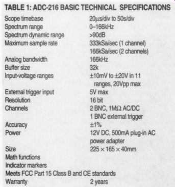
TABLE 1: ADC-216 BASIC TECHNICAL SPECIFICATION
------------------
Application notes are available that describe the use of the ADC-216 for audio spectrum analysis. These notes give examples for CD player, amplifier and loudspeaker tests. You can plot frequency-response curves using a sine-sweep generator. The ADC-216 data collection and processing is optimized for speed. A 30 second sweep across the audio band allows the ADC-216 to perform hundreds of FFTs. Crosstalk measurement is also Very easy.
Manual
The ADC-216 is a new product for Pico. The manual I received with the unit was for the ADC-200, which is a different 8 bit device. It is printed in four languages, with just seven pages of English-language content. Only one page covers actual operation, which is enough to get you going. Fortunately, the ADC-216 is very easy to use. The PicoScope program has an extensive help file that explains all the details of operation, including the extensive customizing features for production lab testing. There is also an on-screen guided tour.
I put the ADC-216 through the same type of tests as the PCS64i, keeping with in its lower bandwidth and voltage limits. I repeated some of the figures so you can see the differences, but keep in mind that these two units have different missions. The PCS64i is an 8-bit high-frequency general-purpose DSO, and the lower-frequency 16-bit ADC-216 is optimized for audio testing.
PicoScope allows you to simultaneously display the scope, spectrum analyzer, and digital multimeter (DMM) views, tiled or cascaded. The Meter view can measure DC volts, AC volts, dB, or frequency. Clicking on any one of the three screens makes it active, and they can be maximized to fill the window.
DSO (Oscilloscope) View
The oscilloscope program boots in the DSO mode and uses a Windows format with pull-down menus to set all the parameters. The scope display uses a 10 x 8 division grid (Fig. 19) that you can turn off. You can set the vertical input for each channel to Auto mode, where it selects the lowest input level that avoids clipping. It can also be set manually from full ranges of +/- 10mV to +/- 20V. This differs from the usual mV/div settings on a conventional scope.
You can set the timebase from 20us/ div to 50s/div, and the selected time/div and voltage range for each channel are shown on a status bar above the scope display. You can zoom the vertical range from x1 to x100, and the timebase range from x1 to x200. When you zoom the timebase, a horizontal scroll bar appears that allows you to move beyond the ten displayed horizontal divisions.
Operation of the DSO is completely intuitive. The two channels share a single multiplexed 16-bit ADC. The sample rate, and thus the analog bandwidth, are halved when you engage the second channel. Even so, the minimum band width is 166kHz at 166kSa/s. The screen update is not quite as fast as the PCS64i, but the 16-bit precision is worth the wait. In Auto mode, some additional time is required to step up through the volt age ranges. The waveforms have a smoother appearance, with blue and red traces (channel A and B) on a white background. You can date stamp the screens and add test notes.
You can save any waveform on the screen in a proprietary Pico file format (psd). You can also use Copy as Graph in the Edit menu to paste the view in another document. I was able to cut and paste the graph into a number of Windows programs such as Word, Power Point, and Excel. The Copy as Text option, also in the Edit menu, generates an ASCII table that lists the data points, as well as the time- and voltage-step scaling factors for the data. This data can be imported into Excel for numeric manipulation. This is also the method used to update the THD tables in the PicoTHD program.
Input Ratings
Each input is rated for +/- 20V p-p (AC + DC) max. Excessive input voltage can damage the ADC-216 interface unit, or conceivably even your computer if the voltage is high enough.
As with the PCS64i, I tried a number of signals on the ADC-216 to assess its limits. Two full cycles of the 1kHz square wave from my function generator were just about perfect, as you can see in Fig. 19. (This is a PrintScrn capture. The later figures without the Windows border make use of the program's Copy as Graph function.) Switching to two channels did not degrade the display resolution.
With the timebase set for 100us (one cycle displayed), I was able to zoom the stored 1kHz image x200 (500ns/div). At this extreme, I measured the square-wave rise time to be 3ns. When I switched be tween timebase and voltage ranges, the update time was less than one second.
I decreased the square wave frequency to 100Hz, 10Hz, and 1Hz, adjusting the timebase accordingly, and the wave form was square in these ranges. Using the fastest 20us/div timebase, two cycles of the 10kHz square wave were again perfect. When I turned on the second channel, there was a bit more slope to the vertical transitions, but still with very square corners.
At the 166kHz limit, using the fastest 20us/div timebase and the zoom feature, the square wave became a triangle (Fig. 20), although the peak amplitude was still correct. The function-generator tri angle waves had nice sharp points on the peaks, with straight transitions.
Accuracy Checking
To check accuracy, I fed the ADC-216 a low-distortion 6.4V RMS 1kHz sine wave from the oscillator of my HP339A distortion test set, with the DSO set to Auto and 200us/div. I used the markers to mea sure the positive and negative peaks of the sine wave and the time span of two zero crossings. The peak-to-peak dV was 17.98V. The markers are activated by a mouse click/drag, and you can drag or step them with the keyboard cursor arrows. You set the left marker with the left mouse button and the right marker with the right button. The value of each marker and the difference between them is displayed on the scope screen. The Delete key removes the markers after you highlight them.
The dT reading was 1007ms. I used the Meter view to check these markers.
It read 6.36V RMS and 991Hz, which is within the 1% accuracy spec for the ADC-216. The marker functions in con junction with the Meter view allow you to cross-check your measured data.
Next I increased the timebase to check for aliasing. At 2ms/div the width of the 20 displayed cycles was accurate, but the amplitude peaks just started to vary. Visible amplitude modulation started at 5Sms/div. At 50ms/div, the amplitude had decreased markedly, but the time between zero crossings remained 1-ms up to 100ms/div. At 200ms/div the display went flat to noise.
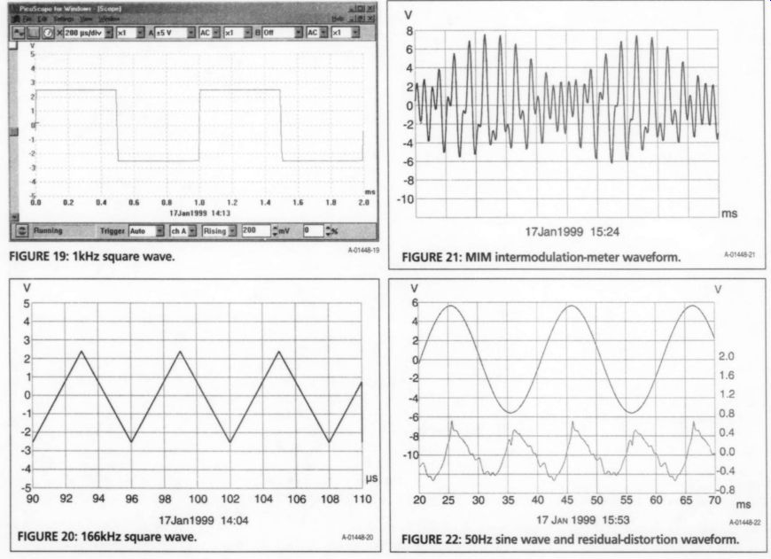
Fig. 19, FIG. 20: 166kHz square wave. FIG. 21: MIM intermodulation-meter waveform. FIG. 22
The ADC-216 handled the complex but repeatable intermodulation distortion (IMD) meter waveforms very well.
The 9kHz + 10.05kHz + 20kHz MIM signal is shown in Fig. 21. The display is al most as good as an analog scope, and you can see the effect of better digital resolution when compared with Fig. 6 in Part 2 (yes, all these comparisons are a bit un fair to the PCS64i, which does an excellent job, given its 8-bit ADC).
For the final DSO test, I ran a 1kHz, 4V RMS sine wave from my function generator through the HP339A. The upper trace in Fig. 22 is the fundamental, which measured 0.57% THD+N. The lower waveform is the residual distortion signal (not to scale) after passing through the -100dB notch filter. You can clearly see the second harmonic, along with the lower amplitude fourth. The 80kHz low-pass filter in the HP339A re moves the really high harmonics, so as a result, Fig. 7 (Part 2) comes off looking almost as good. All the math functions work in both real time and with stored waveforms.
Triggering Modes
The ADC-216 trigger also works like an analog scope, with edge triggering on either the rising or falling edge in one of the two channels, or the external trigger input, limited to 5V maximum. The DSO has a conventional free-run mode, and the triggering must be turned on to get stable waveforms.
A Trigger Level menu allows you to set the level in increments of as little as 1mV, depending on the selected level. You can also enter a specific voltage level in the window. A convenient marker at the left edge shows the trigger-level point. Since the vertical position is done in software, this trigger level is not screen-position sensitive. If you move a trace with the vertical-position scroll bar, the trigger level moves with the waveform. This is a very nice feature.
There is another menu that lets you delay the trigger a specified percentage of the total display time, enabling you to 20 back in time to see the condition that caused the trigger. For troubleshooting problems that occur only intermittently there are Stop On Trigger and Save On Trigger functions that let you run the DSO unattended.
FFT (Spectrum Analyzer) View
The FFT display is that of a spectrum analyzer, with vertical magnitude and horizontal frequency as shown in Fig. 23 (an other PrintScrn capture).
The vertical input uses the same voltage ranges as the DSO mode, and the vertical display can be scaled in volts or dB. The frequency-range selector sets the maximum frequency, which extends over six major horizontal divisions, from 81Hz-166kHz. The spectrum is displayed from zero to the selected frequency, in either linear or log format. There is also a zoom menu that can expand the stored horizontal display up to x20.
The Settings menu allows you to select the number of spectrum bands-either 128 (fastest), 256 (default), 512, or 1024 greatest accuracy). You can use two channels at a time for FFT.
Seven FFT tapers are offered in the Settings menu: Rectangular, Triangle, Gaussian, Hamming, Blackman, Parzen, and Hanning. Two measurement markers are provided, half that of the DSO mode, since the vertical cursor reads both level and frequency. The triggering circuit works on signal amplitude just like the DSO mode.
The FFT vertical axis has a range of 100dBV, which changes with the + volt range. The Auto mode ensures that the I ran a baseline of the +5V-range noise floor by grounding the input in the 1.3kHz range. The average noise floor proved to be -127dB (actually dBr). Now you can really see what those extra eight bits do for you. There was a very small 60Hz power-supply component at -94dB, and the next three harmonics of 60Hz were all below -105dB.
The 3V RMS 50Hz sine wave from the HP339A test oscillator (0.0019% THD+N) shows no significant 50Hz harmonics, and the noise floor is -107dB, as you can see in Fig. 23.
The spectrum of a 50Hz square wave using the 1.6kHz range was perfect down through the 12% harmonic.
Figure 24 shows the same evidence of even order harmonics […] .Next I set the function generator for a 3V RMS 50Hz sine wave, which measures 1.03% THD+N on the HP339A. I recorded the FFT spectrum with the Hanning taper, as shown in Fig. 25 (see the earlier Fig. 13 in Part 2 for comparison). I captured the PicoTHD-program data table that shows the magnitude of the fundamental and its first five harmonics in dB, and the total THD (in dB or percent). The table also lists SINAD (signal, noise, and distortion for FM receiver tests), the spurious free dynamic range (SFDR), and the FFT taper frequency spread percentage.
You must use the Copy as Text function to update this table if you change any input or FFT parameter.
Figure 26 is the spectrum of the 9kHz + 10.05kHz + 20kHz MIM intermodulation meter waveform at 3V RMS. The FFT is set to the 20.8kHz range here. The 1kHz marker where the IM measurements made (markers are not captured by Copy as Graph) showed -79dB. The spectrum is more detailed than Fig. 17 Part 2), with a number of harmonics hat were previously hidden in the higher noise floor.
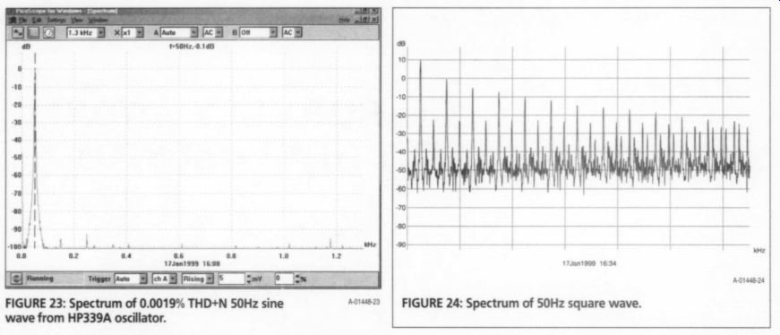
FIGURE 23: Spectrum of 0.0019% THD+N 50Hz sine wave from HP339A oscillator. FIGURE 24: Spectrum of 50Hz square wave.
Data Recorder Program
Since the PicoLog program is similar to he PCS64i transient recorder mode, I did not repeat this test on the ADC-216.
It has extra functions, such as display and data-limit alarm without recording, Realtime, and Fast recording.
Conclusion
The ADC-216 is a significant jump in PC based DSO technology. Its 1% accuracy and 90+ dB of dynamic range are comparable to those of a high-performance Lab DSO. The ADC-216 is also a precision audio test instrument, with advanced capabilities and custom features if you wish to develop your own software. The Auto mode makes it foolproof during spectrum measurements. At $800, it is a good value, and I highly recommended it.
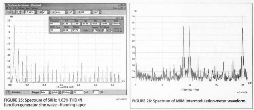
FIGURE 25: Spectrum of 50Hz 1.03% THD+N function-generator sine wave-Hanning taper.
FIGURE 26: Spectrum of MIM intermodulation-meter waveform.
--------
Also see: