In the majority of am-fm broadcast installations today, transmitter and studio operations are combined. However, in the event of transmitter problem revealed the remote-control monitoring devices, the duties of the personnel often become divided--those concerned with studio maintenance and those concerned with transmitter maintenance.
In any event, it is desirable from an orientation standpoint to treat transmitter installations as a separate, but correlated, study from studio installations. In the instance of remote control from the studio, it is still the responsibility of the operator to analyze any malfunction, to remove the transmitter from the air if it is out of tolerance (this is automatic in many instances), and to place the standby transmitter (or the properly operating portion of a parallel transmitter) on the air.
During the regular broadcast day, the transmitter operator keeps the circuits properly tuned, maintains correct power input to the final stage, logs meter readings in accordance with current FCC rules ( which also aids in forestalling trouble), checks the frequency, and maintains the modulation at a level consistent with good engineering practice and the type of pro gram in progress.
The first discussion to follow will pertain to the all-important operation of the broadcast transmitting installation in order to achieve the best results possible from the finely engineered equipment available and in use today.
Operating practice at the transmitter is just as important to the final result of overall performance as it is at the broadcast studio. The operation of the transmitter and associated speech-input equipment may be shown to be a highly specialized art, and we have chosen the term "operational engineering" to define the content of the special study undertaken in this part of the Section.
Following the operations sections, the testing and maintenance of transmitting equipment will be discussed. Proof-of-performance measurements are detailed, and a suggested preventive-maintenance routine is given.
14-1. OPERATOR'S DUTIES
It is true that the primary purpose of the transmitter operator is to keep the station on the air. But with the increased demands for higher-fidelity program transmission, the day when a typical "ship operator" possessing thorough technical understanding could step into a broadcast installation has passed. The operator of a broadcast transmitting plant has a specialized range of duties requiring a technical education as well as a thorough under standing and appreciation of the more intangible values of program material.
A number of his fundamental duties are, of course, strictly technical in nature. In brief, they consist of turning on the transmitter before the beginning of the daily program schedule, checking all meter readings to make proper adjustments, checking level with the studio, shutting down the transmitter after sign-off, repairing and maintaining equipment, and testing for noise and distortion levels. During the daily operating schedule, he consistently monitors the program with a monitoring amplifier and speaker, adjusts line-amplifier gain in accordance with good engineering practice pertaining to percentage modulation ( the transmitter operator does not normally "ride gain" as does the studio operator), maintains correct transmitter tuning, logs all meter readings as required by the FCC, and corrects any trouble that develops in the shortest possible time in order to keep the station on the air.
The transmitter operator in all but the lowest-power local stations is usually scheduled to be on duty at least 30 minutes prior to air time for the purpose of getting the equipment ready for the broadcast day. The start of an operator's day ( when on duty in person at the transmitter) may be outlined as follows:
1. Power is applied to the audio rack, including such measuring equipment as the frequency and modulation monitors. The audio line is used as a program loop and opened by inserting a patch cord into the line jacks. This removes the line from the input to the line amplifier and prevents any test program that might be on the line from the studio from being applied to the transmitter when it is first turned on.
2. A visual inspection of all relays in antenna-phasing cabinets ( where used) and in coupling houses at the antenna is performed. Relay armatures are manually operated to ascertain freedom of movement.
All rf meters are observed for bent hands or zero set.
3. An inspection of all safety gaps is carried out, including antenna and transmission-line lightning gaps for approximate correct spacings.
4. Air-cooling systems usually start the blower motors when the filament-on switches are operated. Transmitter filaments are next turned on and filament voltages checked. Minimum voltage should first be applied to large power tubes that have tungsten-type filaments; then the voltage should be run up to normal after about 3 to 5 minutes.
This procedure is automatic in some transmitters and helps to lengthen the usable life of such power tubes. Tubes with thoriated tungsten or oxide-coated filaments, such as those used in the low-power stages, are always operated at normal filament voltage for maximum tube life.
5. Plate voltage can then be applied to low-power units or exciter units (power installations of 1 kW or more) to check for proper excitation to the final stage.
6. Low power is then applied to the final stage. All meter readings are checked for normal low-power operation. If everything is normal, high power is applied and meter readings are checked.
7. Filament and line voltages are checked and adjusted for high-power operation. Final adjustment is made on the final stage for optimum meter readings regarding resonance and power input.
8. Since the control-room operator sometimes has circuits "hot" with his own testing procedure, the transmitter operator plugs a patch cord from the program line to a monitor amplifier to ascertain continuity of the program line.
He then notifies the control operator to stand by for an overall circuit test. When this has been done, the transmitter operator removes the patch cord, automatically restoring the input line amplifier. A test tone may then be fed from the studio to check the overall continuity of the circuits from the studio to the transmitter modulators. In the event of remote-control operation, the studio operator has full control over the transmitter input.
Level checks with the studio are not required as a daily procedure after an initial installation has been made, tested, and operated for some time, since with properly operating equipment the level remains nearly the same over a period of time. At regular intervals, however, it is desirable to use a signal generator to check the frequency characteristics of the line and transmitting equipment. In this connection, it is advisable for the transmitter operator to understand the difference in modulator power requirements for sine waves and the complex waveforms of speech or music program content.
It will be remembered from circuit theory that for a class-C modulated amplifier the power requirement for complete sinusoidal modulation is 50 percent of the dc power input to the modulated tube or tubes. Fig. 11-8 (Section 11) shows how the peak factor of speech or music waves varies greatly from that of a pure sine wave, when "peaked" the same on a VU meter. This peak factor of program waves is 10 to 15 dB more than that of a sine wave. That is, the ratio of peak to rms voltage is far greater for complex waveforms than for sine waves. The average power for complete modulation of a transmitter over a period of time is far less than the aver age power required for complete modulation by means of a signal genera tor. It is a well known fact that for program signal waves the modulator power required may be 25 percent or less of the dc power input to a class-C stage. Therefore, if a signal generator is used at the studio for frequency runs or level checks, the transmitter operator must realize that if he adjusts the gain on the line amplifier to give 100 percent modulation on sine waves, the same adjustment will be 10 to 15 dB high for program signals.
The gain adjustment must be lowered accordingly to the point that experience has dictated for program modulation before the actual program schedule starts. In the past, this has led to some confusion among transmitter operators.
This difference in peak factor between program and sine waves is also noticed when comparing the percent of antenna-current increase with 100-percent modulation. It is true that the antenna-current increase should be approximately 22.5 percent over no modulation when a sine wave is applied to the transmitter at 100 percent modulation. Antenna current increases for 100 percent program modulation, however, will be much less, due not only to the difference in peak factor, but also the sluggishness of the thermocouple rf meter action. This slowness of action is due to the heating effect of the two dissimilar metals on which the action of the meter depends.
14-2. CORRELATION OF METER READINGS
It is only natural that the program level being sent by wire from the studio be of utmost importance from a strictly operational point of view to the transmitter operator. With competent studio personnel, the line-amplifier gain adjustment may be set for 100-percent modulation on program peaks at the start of the day and left at that adjustment. Many times, however, a transmitter operator, who in some cases may not appreciate musical and dramatic values, will become piqued with the control operator when the program level is very low. He should realize, however, that broadcast stations are not strictly for "communications," but are intended to bring entertainment into the home with as much of the original content as possible consistent with the state of the art. Certain types of programs, symphony concerts in particular, are meant for those listeners in the primary service area and not intended to override the noise level at some secondary service point. If the monitor speaker is turned up in volume consistent with that of the interested listener at home for these types of programs, the transmitter operator will be able to use good judgment as to whether the signal is or is not entirely too low in level to be usable for proper modulation.
Program Levels
In relation to the study of program levels, it is of primary importance to understand the characteristics of the indicating meters used at both ends of the transmission system. These meters differ in characteristics because of the different functions which they are intended to perform. The standard VU meter, used in most broadcast studios today, is an rms-indicating full-wave rectifier device intended to give a close visual approximation of the sound waves emanating from the speaker. However, the concern at the transmitter is with modulating voltages, and a semi-peak indicating device is necessary and required by the FCC. If peaks of the program signal con tent should be excessive and occur in rapid succession, danger of circuit component breakdowns would arise as well as severe adjacent-channel interference. Therefore, since the peak factor of program waves is high, the modulation meter is a peak-indicating device. It is also necessary that a phase-reverse switch be incorporated in the modulation-meter circuit to switch the polarity of the input to the metering circuit so that either the positive or negative side of the modulated envelope may be monitored separately. Thus, it is obvious that there are two distinct types of level meters, namely, a full-wave rms meter at the studio and a half-wave peak meter at the transmitter. In addition to these meters, there is a limiting-type amplifier (in most modern installations) which is used at the transmitter as a line amplifier. This has meters which measure the amount of compression ( full-wave peak meter) and output level in VU ( full-wave rms meter).
The number of different types of indicating meters should not confuse the operator as long as the proper interpretation is given to the readings.
Fig. 14-1 shows the indication of a program peak at a given instant on the various meters involved. The studio VU meter has registered 100; the compression meter at the transmitter shows the normal 5-dB limiting; the line-amplifier output meter shows 100; and the modulation meter would show either 100-percent modulation on positive peaks or, if set to monitor negative peaks, might show only 60-percent modulation. This, of course, could be just reversed with a change in polarity of the microphone output or any connection in between.
It is a well known fact that speech waves are not equal in positive and negative peaks regardless of the type of microphone used. This may be observed from the graph of the speech wave shown in Fig. 14-2. Two speakers working from opposite sides of a bidirectional microphone and peaked the same on the studio VU meter will not give equal indications on the modulation meter when it is set to indicate a certain peak (either positive or negative) because of the negative-peak effect.
Assume, for example, that the modulation-monitor switch is set to monitor the negative peaks, and the indication of one voice is close to 100 percent. The indication of the voice on the other side of the microphone (therefore of opposite polarity at the microphone output transformer) may indicate only 40 to 50 percent, with the amplitude of the studio VU meter remaining the same. For this reason, it is obvious why misunderstandings sometimes arise between studio and transmitter personnel regarding the comparative levels of two or more voices.
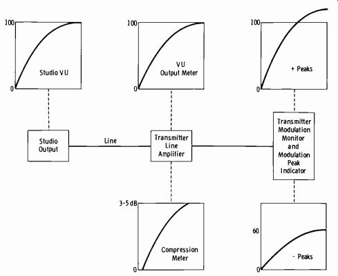
Fig. 14-1. Indications of a given program peak on several meters.
What indication exists at the transmitter plant to show a true indication of comparative levels from the studio? It has been shown that the half-wave reading of the modulation meter, which depends on the polarity of operation, is not a true indication of comparative levels from the studios. The VU meter at the output of a limiting amplifier would not be a true indication since the output level is limited by the compression taking place in the amplifier for signals over a predetermined level. The compression meter, although a full-wave indicating device, is a peak-reading instrument, and, since the peak factor of program waves varies considerably, it is not an absolutely accurate indication of comparative levels. It is, however, the most reliable indication (within limits) existing at the transmitter, since it is full-wave rectified and is limited by only wire-line characteristics. If two voices, for example, show about the same amount of compression, the comparative levels (not loudness) may be considered very nearly the same.
100-Percent Modulation ( AM)
Fig. 14-3A shows an oscillographic pattern of a carrier modulated 100 percent by a sine-wave tone. This illustration shows what constitutes positive and negative modulation of the carrier. It may be seen that negative, or trough, modulation cannot attain more than 100 percent of the avail able range, whereas positive, or peak, modulation may go over 100 percent.
When a carrier is thus modulated with a pure tone, the degree of modulation is:
m Eav- Emin=
Eav where, m is the degree of modulation, Ea, is the average envelope amplitude, E,n1,, is the minimum envelope amplitude.
0.001 Sec
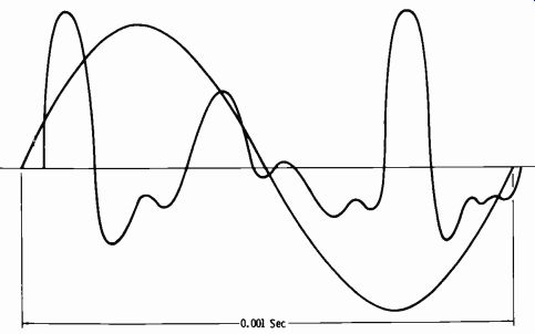
Fig. 14-2. Curves indicating peak factors of voice and sine waves.
The peaks and troughs of the envelope will be equal. When the minimum envelope amplitude (negative peak modulation) is zero in the foregoing equation, m is 1.0, and the degree of modulation is complete, or 100 percent expressed in percentage modulation.
When the envelope variation is not sinusoidal, such as is true for pro gram signals, the positive and negative peaks will not be equal, and the percentage of modulation differs for the peaks and troughs of modulation as follows:
Positive peak modulation = E°'" Ea° E"° 100
Negative peak modulation- Emit' 100 where, E"° is the average envelope amplitude, Emi" is the minimum envelope amplitude, E. is the maximum envelope amplitude.
Thus, it is possible to understand why the trough modulation cannot exceed 100 percent, since the minimum voltage cannot be less than zero. It may be seen, however, that the positive peak voltage may be more than twice the average (or carrier) voltage, in which case the positive peak modulation will exceed 100 percent. What important information does this hold for the transmitter operator? First, it should be clarified in the operator's mind that overmodulation can take place on the negative ( trough) modulation as well as on the positive (peak) modulation. It is true that the degree of modulation can never exceed unity on the negative peaks, but it can exceed unity on the positive peaks. Complete modulation (of a class-C stage) , however, requires that the peak values of the modulating voltage equal the dc plate voltage of the modulated stage. Fig. 14-3B shows an oscillographic pattern of a carrier wave with modulating voltage exceeding the dc plate voltage and causing overmodulation of the carrier. It is true that the positive modulation peaks exceed unity while the negative peaks are cut off by the excessive negative modulating voltage and cannot exceed unity. This excess energy, however, which allows the voltage applied to the rf-amplifier plate circuit to become negative with respect to ground, causes radiation in the form of spurious frequencies, resulting in "splatter" and adjacent-channel interference.
Positive Negative
(A) 100 % modulation. (B) Overmodulation.
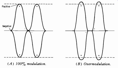
Fig. 14-3. Modulation envelopes.
This actually is overmodulation in its severest form, since positive peaks may extend beyond 100-percent modulation without amplitude distortion, whereas clipping of the negative peaks will cause severe amplitude distortion. It will be remembered that the bandwidth occupied by the carrier and sidebands depends ( for amplitude modulation) not on the degree of modulation, but on the highest frequency being transmitted. Amplitude distortion resulting from negative-peak overmodulation generates a number of distortion harmonics that may extend high enough to spread the sidebands into adjacent channels.
This discussion has been presented in order to show the transmitter operator that the negative side of the modulation is the most important peak to monitor on the modulation meter. It should be held under 100 percent at all times. It is well to remember that a modulation meter of the vacuum-tube-voltmeter type will not be able to indicate over 100 percent (negative) on the meter because the peaks cannot attain more than this value. This is why an oscilloscope is sometimes used at a broadcast transmitter to show negative peak overmodulation, since the negative peak clip ping shows up as white lines across the center of the modulated pattern.
When the usual vacuum-tube-voltmeter type of modulation indicator is used, the flasher should be set for 95-percent modulation so that the warning is given usually before the meter ever swings to this value. A flasher will respond on a much faster increment of program peaks than will the indicating meter movement.
NOTE: FCC rules at the time of this writing limit positive peak modulation to 125 percent. Always check current FCC rules.
FM Modulation-Monitor Interpretation
Peak amplitude variations in the positive and negative directions show up on an fm transmitter monitor as a decided difference in amplitude of the plus and minus excursions of the meter. In this case, however, we are not concerned with either peak in relation to distortion, since modern fm transmitters are able to over-modulate greatly either plus or minus without inherent distortion. Distortion does occur, however, in the receiver when overmodulation over noticeable periods of time occurs, since few receivers have the capability of providing faithful reproduction of a modulating signal that produces a frequency swing much in excess of the maximum of 150 kHz (-x-75 kHz, which is defined as the value of 100-percent modulation for fm broadcasting).
The fm transmitter operator, therefore, is concerned with preventing overmodulation on either peak. For this reason, it is of utmost value to have all studio microphones connected so that their maximum polarity occurs on a definite side, either plus or minus on the modulation monitor. Otherwise, the transmitter operator must check his peaks at each change of microphone before he is certain that the maximum peaks are not over 100 percent.
Automatic Correction of Nonsymmetrical Audio Peaks
The problem of peak polarity in proper modulating techniques, particularly important in AM transmission, has been stressed. A special passive device designed to distribute equally nonsymmetrical audio peaks, particularly those produced by certain inherent characteristics of the human voice, is shown in Fig. 14-4. By removing asymmetrical energy, this unit permits higher average modulation, thus giving the effect of higher transmitter power with no change in the program signal level.
Courtesy Kahn Research laboratories, Inc.
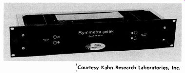
Fig. 14-4. A device for removing asymmetrical energy from audio peaks.
Long-line telephone circuits normally correct for speech asymmetry, and music seldom contains unbalanced waveforms. Thus, asymmetrical modulation peaks are mainly caused by live or tape-recorded voice programs originating locally or over relatively short telephone lines. Since the main purpose of this device is to distribute nonsymmetrical energy equally with out disturbing symmetrical sources, the remaining modulation problem is thereby removed. Local voice program levels can be raised to equal those of other programs without danger of overmodulation.
This unit also offers another advantage for users of compressor, limiter, or uniform-level type amplifiers. With reduced peak energy, limiting will take place only during higher average modulation levels. When speech clippers are employed, the unit removes the low-frequency bounce normally produced by dc shifts in clipped nonsymmetrical waves.
14-3. LIMITER AMPLIFIERS
The limiting amplifier, or compression amplifier, is a very important link in a broadcast installation. However, its effect may not be advantageous if the wrong operational interpretation is given to the main purpose for which it is designed. This type of amplifier, as designed for use in a broad cast installation, is intended as a peak limiting device, the amount of gain reduction being a function of the program peak amplitude. In order to prevent material reduction in the dynamic range of the signal, the peak gain reduction should not be more than 3 to 5 dB. A broadcast limiting amplifier, therefore, should not be considered as a volume limiter, but as a peak limiter intended to prevent adjacent-channel interference and over loading of transmitter components.
In some installations, a special agc amplifier is used for automatic announcer override of musical background. In this application (which can be considered a small step toward automation) , the normal program reaches the agc input at -35 dB, for example. The announce circuit has added amplification ahead of the agc amplifier so that the signal is at a level of -20 dB, for example. Since the agc tends to hold the output constant, about 15 dB of program reduction occurs so that the announce portion is at normal level and gain riding of background is not necessary. The reader should bear in mind that the main limiter amplifier has a normal limiting of only 3 to 5 dB and is not to be confused with the operation previously noted, where the actual compression of the announce portion may be as much as 15 to 25 dB.
It is true that doubling the output power of a transmitter raises the signal intensity 3 dB. It is also true that the limiter amplifier raises the signal level about 3 dB on program peaks. To those familiar with volume indications of program circuits, however, this 3-dB increase on speech or music is of small consequence. As far as the transmitter is concerned, the operator should think of this amplifier as a protective device to limit peaks caused by line transmission and those program peaks that escape the action of the control-room operator.
That the primary purpose of a limiting amplifier may be defeated by erroneous operation is a very important fact for the broadcast operator to know. Seriously detrimental effects will result if this amplifier is operated as a volume-compression device to attempt to provide a coverage area greater than a given power and transmitter location warrant. The attack time of peak limiting (about 0.001 second) is determined by a resistor-capacitor charging circuit with the inherent characteristics of a low-pass filter. At high frequencies, and where the duration of the peak is short compared to this operating time, a portion of the peak energy will escape limiting action. If the average signal level is so high that a great amount of compression takes place at all times, a larger amount of adjacent-channel interference will result, defeating one of the main purposes of the amplifier.
This has been quite noticeable in practice when the program content consists of music from dance orchestras of brass instruments where high peak powers at high frequencies are prevalent. A limiting amplifier operated properly for broadcast service will show about 3 to 5 dB of intermit tent gain reduction as indicated by the peak-reading meter used to show the amount of program peak compression. The operator must realize that for certain types of programs, such as symphonies, liturgical music, and operas, the average audio signal may be very low over a period of time-even with limiting amplifiers in use. Dynamic range is just as important to high fidelity transmission of these types of programs as is the frequency range. Another consideration is the recovery time, or time required to restore the gain to normal after a peak has momentarily reduced the gain. Optimum recovery time varies for different types of program material. Piano music, for example, sounds unnatural when the recovery time is too short, because the effect is similar to inadequate damping of the strings after they are struck or to holding the sustaining pedal too long on the loud notes.
As the recovery time is lengthened, however, the gain will be reduced (in effect) a greater proportion of the total time, and unnatural transmission of certain passages in music will result. If limiting amplifiers are operated properly and not subjected to more than the specified amount of peak load, however, they will serve their primary purpose quite satisfactorily without introducing undesirable effects.
When thinking of a compression amplifier as a means of increasing the service area of a transmitter, keep in mind the known facts concerning the psychological differences that exist in listening habits for various types of programs. A lower relative signal level is tolerable for dance music, news broadcasts, etc., where the average audio level is high over a period of time.
In this case where listeners well outside the primary service area of the station may be numerous, the maximum amount of peak limiting may be used to help raise the signal-to-noise ratio at the receiving point. However, symphony broadcasts, choral music, certain liturgical music, opera, etc., where the average audio signal may be very low over a period of time, will appeal only to those listeners who are adequately served with strong carrier signals. In the interests of preserving the original dramatic effects of this type of program, it simply is not technically feasible for a broadcaster to attempt to set a fixed value of coverage area for all types of program material. Similarly, the engineer responsible for the transmission of programs should not attempt to operate all equipment in the same manner regardless of the type of programs being transmitted.
14-4. ANTENNA IMPEDANCE AND TUNING ( AM)
When an antenna is properly tuned, the reactive component is cancelled, leaving only the resistive component. The power input is the magnitude of the square of the rf current times the antenna resistance in which the current is measured. The antenna resistance is determined during the original installation and is part of the data filed with the FCC. This should be checked at periodic intervals.
There are two basic methods of measuring the antenna impedance, the rf-bridge method and the substitution method. In general, a greater degree of skill is necessary in using the rf bridge than in using the substitution method. However, the bridge method is more accurate and reliable. It re quires becoming thoroughly acquainted with the particular bridge used. It is highly desirable to obtain initial guidance from an experienced user of the bridge.
Bridge Method
Fig. 14-5 shows the equivalent circuit of a shielded rf bridge such as is used for antenna work. The rf impedance is measured either by a substitution method on the bridge (not to be confused with the substitution method without a bridge as described later) or directly by the unity-ratio bridge method.
Bridge Input From RF Oscillator Note: Capacitors with dashed connections represent capacitance of shield.
Fig. 14-5. Equivalent circuit of shielded rf bridge.
Method 1 (Bridge-Substitution Method)--The unknown impedance is placed in parallel with C5R5. Then R8 is adjusted to zero, and Cs is adjusted to some convenient value. The bridge is then balanced ( zero output at the output terminals) with a convenient resistance and capacitance in the X arm. The unknown impedance is then removed. The resistive and reactive components are now determined from the changes required in the calibrated Cs and Rs controls to restore the balance. Obviously, in the use of any bridge, the manufacturer's instructions and precautions must be followed carefully.
Method 2 (Unity-Ratio Bridge Method)
The bridge is first balanced with Rs shorted to ground. The balance is made by adjusting Cs or by the use of an external capacitance from terminal A or C to ground as required.
The unknown impedance is then connected to the X arm. The bridge is again balanced by adjusting C8Rs to match the unknown impedance, indicating the resistive and reactive component values. With this particular type of bridge, when the unknown impedance is inductive, it must be made capacitive by shunting it with a known capacitance (shown in Fig. 14-5 as C') so that balance may be obtained by the capacitance in the standard (S) arm.
Refer to Fig. 14-6 (T section of a single-antenna tuning unit). The reactance values for the circuit can be calculated as follows:
X1 = +-VR1R2 X2=+VR1R2 X3=-VR1R2 where,
X1 is the reactance of L1, X2 is the reactance of L2, X3 is the reactance of C, R1 is the line impedance, R2 is the antenna resistance.
R1 LI A
Fig. 14-6. Representation of single T section, antenna tuning unit.
First, it is necessary to determine the impedance of the antenna at the operating frequency so that the proper values of the inductance and capacitance arms may be computed. Impedance measurement of the antenna is made directly at the antenna-tower input terminal with the line disconnected. Usually, measurements are made at frequencies above and below the operating frequency, and the resistance at the operating frequency is determined from a graph of antenna resistance versus frequency.
As an example, suppose a tower has a height of 190 electrical degrees and 28 ohms of resistance and +j25 ohms of reactance. The transmission-line impedance is 70 ohms. Substitution of these values in the preceding equations gives:
- /(70) (28) _ x/1960 = 44 ohms (approx)
Therefore, X1, X2, and X3 should have a value of 44 ohms at the operating frequency.
The antenna reactance in this case is +j25 ohms. It is assumed that this reactance is a part of the value of X2. Therefore, subtract the 25 ohms of positive antenna reactance from 44 ohms, giving 19 ohms to be obtained in X2. When X1 and X3 have been adjusted to 44 ohms, an impedance match is produced between the transmission line and the antenna resistance. Adjustment of X2 to 19 ohms cancels the antenna reactance, which would cause a loss of efficiency and a high vswr.
The rf impedance bridge is used in making these adjustments by connecting it across the input of the matching network with the transmission line disconnected. When measurements indicate that an input impedance of 70 ohms has been obtained (with antenna connected), the transmission line is reconnected for the final check before applying power from the transmitter.
Care should be taken that the capacitive branch uses capacitors having a high enough current rating to withstand the current at that point. Usually two or more capacitors of the proper value (to total the required value) are used to handle a current larger than one could safely carry.
Substitution Method When an impedance bridge cannot be obtained for the necessary length of time, a method commonly known as the substitution method is used to tune the antenna system. Fig. 14-7 shows the arrangement of coupling circuit and tuning unit necessary for this procedure.
Fig. 14-7. Substitution method for adjusting antenna system.
It may be seen that it is necessary to switch the line from the tuner to a substitution resistance, which should equal the line impedance, so that a change in line current indicated by the meter (M) is noted when the switching action occurs. The tuner is properly adjusted when no change occurs.
Obviously, full power must not be applied to the line, since the voltage rating of a nonreactive resistor is comparatively low. Therefore, connections must be made from a low-power stage in the transmitter, or an accurate rf oscillator may be employed.
Capacitor C is first tuned for a maximum current reading in the line meter (M) with the switch in the resistor position. The tuner input is then switched in, and C is adjusted again for maximum line current. The change in the capacitance of C indicates whether the antenna circuit reactance is capacitive or inductive. If it is necessary to increase the capacitance, the load is capacitively reactive. Conversely, if the capacitor must be de creased to increase the line current, the load is inductively reactive. If no change in C is necessary, the load is resistive.
Final Check of Antenna Match
Whichever method of tuning has been employed, a final check of match conditions should be made before full power is applied to the circuits. The measuring equipment is removed, and low-range thermal milli-ammeters are inserted at each end of the ungrounded conductor of the line. Sufficient power is then applied from a low-power stage of the transmitter so that the meters give an adequate reading. When the tuning adjustments are correct, these readings agree within 15 percent, showing a proper feeding match between the line and tower networks.
14-5. FIELD-STRENGTH MEASUREMENT TECHNIQUES ( AM)
The inverse field is the un-attenuated ground wave (the ground-wave field intensity that would exist considering only the effect of distance) and is used for comparison purposes. The rms value of this field is the radius of a circle (Fig. 14-8) which has the same area as the pattern formed by all the inverse-field-strength values at 1 mile in all horizontal directions from the antenna. The inverse field is found by taking measurements of the actual attenuated field with a field-strength meter; this information is then used to determine the un-attenuated field strength at 1 mile in the direction of each radial. The rms value is then:
E = E102 + E202 + ... + E3002 36 where, Fe is the field strength,
E10 is the field strength at an azimuth angle of 10° (un-attenuated) ,
E20 is the field strength at an azimuth angle of 20°, etc.
Less computation is involved if the actual field is first plotted on polar paper and a polar planimeter used to determine the equivalent-area circle.
The unattenuated ground wave is inversely proportional to the distance and proportional to the square root of the power. Thus if 100 mV/m is produced at 1 mile with 1 kW, 5 kW will produce times 100 mV/m, or 223.5 mV/m from the same antenna.
Fig. 14-8. Inverse field.
Fig. 14-9. Block diagram of a field-strength meter.
Fig. 14-9 is a fundamental block diagram of a field-strength meter. A loop antenna into which a known oscillator amplitude may be injected for calibration of the meter is normally employed for AM measurements. The measurement of the received signal may be taken from the calibrated attenuator and/or gain controls. Most of the later meters for standard AM frequencies are designed for direct reading in millivolts per meter or microvolts per meter. It is obviously essential to become thoroughly familiar with the equipment before field-strength measurements are attempted.
The following requirements govern the taking and submission of data on the field intensity produced. First, have available a sufficient quantity of log-log graph paper. For a direct match to the FCC Documentary Graphs use K&E Ground-Wave Field Intensity paper No. 61729. Other graph papers that may be used are Dietzgen 3 x 3 cycle log No. 340-L33, or K&E No. 359-120. The steps to be followed are prescribed by the FCC as follows (be sure to check the current rules):
1. Beginning as near to the antenna as possible without including the induction field and to provide for the fact that a broadcast antenna is not a point source of radiation (not less than one wavelength or 5 times the vertical height in the case of a single-element antenna or 10 times the spacing between the elements of a directional antenna) , measurements shall be made on eight or more radials, at intervals of approximately one-tenth mile up to 2 miles from the antenna, at intervals of approximately one-half mile from 2 miles to 6 miles from the antenna, at intervals of approximately 2 miles from 6 miles to 15 or 20 miles from the antenna, and few additional measurements if needed at greater distances from the antenna. When the antenna is rurally located and unobstructed measurements can be made, there shall be as many as 18 or 20 measurements on each radial. However, when the antenna is located in a city where unobstructed measurements are difficult, measurements shall be made on each radial at as many unobstructed locations as possible, even though the number of intervals is considerably less than stated above, particularly within 2 miles of the antenna. In cases when it is not possible to obtain accurate measurements at the closer distances ( even out to 5 or 6 miles due to the character of the intervening terrain) , the measurements at greater distances should be made at closer intervals. (It is suggested that "wave tilt" measurements may be made to determine and compare locations for taking field-intensity measurements, particularly to determine that there are no abrupt changes in ground conductivity or that reflected waves are not causing abnormal intensities.)
2. The required data should be plotted for each radial in accordance with either of the two following methods:
(A) Using log-log coordinate paper, plot the field intensity as the ordinate and the distance as the abscissa.
(B) Using semilog coordinate paper, plot the field intensity times distance as the ordinate on the log scale and the distance as the abscissa on the linear scale.
3. Regardless of which of the methods is employed, the proper curve to be drawn through the points plotted shall be determined by comparison with the curves in FCC Paragraph 73.184 as follows: Place the sheet on which the actual points have been plotted over the appropriate graph in FCC paragraph 73-184. Hold it to the light if necessary and adjust until the curve most closely matching the points is found.
This curve should then be drawn on the sheet on which the points were plotted, together with the inverse-distance curve corresponding to that curve. The field at 1 mile for the radial concerned shall be the ordinate on the inverse-distance curve at 1 mile.
Fig. 14-10. Example of field-strength plot.
Fig. 14-10 shows a typical graph; in this instance the inverse field at 1 mile is found to be 210 mV/m. Dot this in on the 1-mile abscissa and the 210-mV/m ordinate. Since the inverse field varies inversely with the distance, place another dot on the 10-mile abscissa at the 21-mV/m ordinate (one-tenth of 210). The entire inverse curve may then be drawn with a straightedge through these two points.
4. When all radials have been analyzed, a curve shall be plotted on polar-coordinate paper from the fields obtained which gives the inverse- distance field pattern at 1 mile. The radius of a circle whose area is equal to the area bounded by this pattern is the effective field.
5. While making the field-intensity survey, the output power of the station shall be maintained at the licensed power as determined by the direct method. To do this it is necessary to determine accurately the total antenna resistance (the resistance variation method, the substitution method, or the bridge method is acceptable) and to measure the antenna current by an ammeter of acceptable accuracy.
The complete data taken in conjunction with the field-intensity measurements should be recorded, including the following:
1. Tabulation by number of each point of measurement to agree with the map required in item 2 below, the date and time of each measurement, the field intensity (E) , the distance from the antenna (D), and the product of the field intensity and distance (ED) (if data for each radial are plotted on semilogarithmic paper, see above) for each point of measurement.
2. Map showing each point of measurement numbered to agree with tabulation required above.
3. Description of method used to take field-intensity measurements.
4. The family of theoretical curves used in determining the curve for each radial properly identified by conductivity and dielectric constants.
5. The curves drawn for each radial and the field-intensity pattern.
6. Antenna resistance measurement:
(A) Antenna resistance at operating frequency.
(B) Description of method employed.
(C) Tabulation of complete data.
(D) Curve showing antenna resistance versus frequency.
7. Antenna current or currents maintained during field-intensity measurements.
8. Description, accuracy, date, and by whom each instrument was last calibrated.
9. Name, address, and qualifications of the engineer making the measurements.
10. Any other pertinent information.
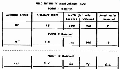
Fig. 14-11. Example of field-strength log for directional antenna.
FIELD INTENSITY MEASUREMENT LOG
A station license may require periodic field-strength measurements (particularly in the case of directional arrays). Even if it is not specifically required, it is a good practice to make these measurements at least quarterly.
The following data are required:
1. Monitor-point identification. On the log for field-strength measurements, this may be only an identifying number. However, a complete description for each point must be on file at the station, usually a duplicate of the original proof-of-performance data filed with the FCC for license application.
2. Specified unattenuated field strength at 1 mile (inverse field) .
3. The inverse field at 1 mile obtained.
4. Actual received field strength at monitoring point logged.
An example of a field-strength log is shown in Fig. 14-11.
It is a good practice to make a complete list of components employed in the antenna system, such as meter types and calibration, types and manufacture of coils and capacitors, etc., along with the actual bridge measurements of reactance for the portions of the coils and (variable) capacitors used. This allows quick replacement and adjustment in case of damage by electrical storms or other causes. Keep a record of all dial settings on a matching or phasing unit. Keep all components and relay contacts clean.
14-6. PROOF OF PERFORMANCE ( AM)
The important characteristics of any modern broadcast installation are an adequate frequency range to convey as much of the original sound as possible, low noise and distortion levels necessary for the required dynamic range, and dependability of performance. One of the most important pieces of auxiliary equipment in the transmitting plant is the instrument used to determine noise and/or distortion over the usable frequency range. Several manufacturers supply such equipment, and most stations are equipped with a means of checking noise and distortion.
Adjustments and maintenance must be performed to assure that the following FCC requirements are met. Always check the latest revisions of FCC rules.
1. The total audio-frequency distortion from microphone terminals to the antenna output, including the microphone amplifier, must not exceed 5 percent harmonics (voltage measurements of arithmetical sum or rss) when modulating from 0 to 84 percent, and not over 7.5 percent harmonics (voltage measurements of arithmetical sum or rss) when modulating 85 to 95 percent. (Distortion shall be measured with modulating frequencies of 50, 100, 400, 1000, 5000, and 7500 Hz up to the tenth harmonic or 16,000 Hz, or any intermediate frequency that readings on these frequencies indicate is desirable.)
2. The audio-frequency transmitting characteristics of the equipment from the microphone terminals (including microphone amplifier un less microphone frequency correction is included, in which event proper allowance shall be made accordingly) to the antenna output must not depart more than 2 dB from the response at 1000 Hz between 100 and 5000 Hz.
3. The carrier shift (current) at any percentage of modulation must not exceed 5 percent.
4. The carrier hum and extraneous noise ( exclusive of microphone and studio noise) level (unweighted rss) must be at least 45 dB below 100-percent modulation for the frequency band of 30 to 20,000 Hz.
Refer to Fig. 2-14 (and associated text in Section 2) for a typical audio-oscillator feed used for a broadcast proof of performance. Remember that this proof requires the signal-generator output to feed a studio microphone preamplifier input.
Fig. 14-12 shows a block diagram of a typical noise and distortion meter, which is also used to check frequency response. In measuring harmonic distortion, the following takes place:
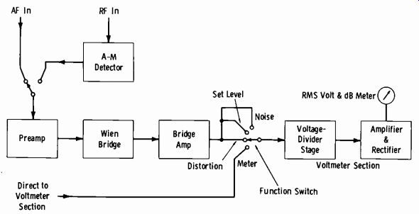
Fig. 14-12. Block diagram of noise-distortion meter.
A. The amplitude of a single-frequency sine wave is measured.
B. A tuning circuit is adjusted to suppress the fundamental frequency.
This is done by a sharply tuned circuit and bridge-balance control to achieve at least 80 dB of suppression at the fundamental frequency.
C. The remaining measured amplitude is the total harmonic distortion.
Normally the transmitter output measurement is taken from a special output of the modulation monitor designed for this purpose. However, an AM detector may also be provided for direct off-the-air measurement as shown in Fig. 14-12.
Always be sure of the "back-to-back" characteristics of the audio oscillator and noise-distortion meter before taking complete proofs or after tube changes or other servicing of the measuring equipment. The direct combination of these instruments should indicate a frequency response flat within 2 dB from 30 to 15,000 Hz. The distortion should measure less than 0.2 percent from 60 Hz to 20 kHz and not more than 0.35 percent from 20 to 50 Hz. The noise should measure at least 70 dB below the output level of the audio oscillator. If it does not, substitute new tubes one at a time (allowing good warmup time) or follow the manufacturers' instructions for necessary adjustments to bring the equipment within the above specifications or the specifications for the particular equipment used.
For frequency-response runs, always consider the back-to-back response of the measuring equipment in calibration of the readings for the input level at the studio. For example, if the back-to-back response is down 2 dB at 5000 Hz relative to 1000 Hz (reference frequency) , then feed an input two decibels higher to the studio at this frequency.
----------------------------
Audio Oscillator
-50 dBm Mic Preamp Amplifier Gain Control Adjusted for 1001%Modulation and Left in This Position for Remainder of Tests All Gains Adjusted for Desired Percentage Modulation of Transmitter All Transmitter Line or STL Terminal Gear Including (Apprac) Limiter Amp for Line at (Limiter Off) 100% Modulation Studio Path From Mic to Output Turn Limiter Section of Limiter Amp Off if Included at Studio.
Bypass Any AGC Amplifier.
Dummy Load Optional RF Pickup for Diode When Included in Noise- Distortion Meter Diode Noise-
Distortion Meter Transmitter Freq Monitor Detector Output Modulation Monitor
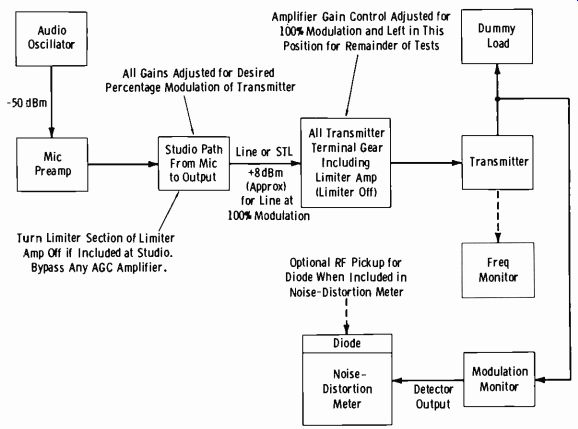
Fig. 14-13. Block diagram of setup for AM proof of performance.
------------------------------
Frequency-Response Runs
Fig. 14-13 shows a typical setup for a complete proof-of-performance run. The FCC rules require an overall response (from studio microphone input to transmitter output) flat within 2 dB from 100 to 5000 Hz. They further require that measurements be made at 25, 50, 85, and 100 percent (or the highest attainable) modulation from 50 to 7500 Hz. A step-by-step procedure follows.
1. With the audio oscillator set at 1000 Hz, feed-50 dBm to a studio microphone input (Fig. 14-13). If the oscillator meter indicates zero dBm at the adjusted gain, the calibrated attenuators will total 50 dB.
Usually the oscillator meter has a full-scale reading of +15 to +17 dBm. It is advisable to adjust the oscillator gain to obtain, say, +10 dBm and set the attenuators for a total of 60 dB to result in a -50 dBm output. Usually the back-to-back measurement previously de scribed gives the best results with this type of operation, particularly when distortion and noise measurements are taken. Usually there are three sets of calibrated attenuators-tens, units, and tenths-so that precise readings may be made.
Courtesy National Association of Broadcasters
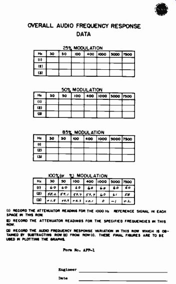
Fig. 14-14. Form for recording
frequency-response data.
2. Adjust the associated faders and master gain control for reference line output (an indication of zero on the studio-line VU meter) . As discussed in Section 2, this is actually +4 to +12 VU. All faders and the master gain control should be in approximately the normal operating positions. The term "approximately" must be used since the microphone-fader setting will in most cases actually be somewhat higher due to the high peak factor of speech waves compared to the sine-wave rms value.
3. Be sure that any agc amplifier is bypassed (patched around) and that if a limiting amplifier is employed at the studio, the limiter section is turned off.
4. At the transmitter, adjust the line or limiter amplifier to obtain 100-percent modulation. The limiter section of the limiter amplifier must be off.
5. Record the oscillator attenuator reading. Refer to Fig. 14-14 for an example of tabulated response data in the form suggested by the NAB (National Association of Broadcasters) . Note that the attenuator reading for 100-percent modulation at 1000 Hz is simply recorded along the entire top row. Assume this to be 60 for illustrative purposes. Copy the figure 60 also in row 2 for 1000 Hz.
6. Tune the oscillator to 30 Hz, and readjust the attenuators (if necessary) to again obtain 100-percent modulation. Record the new attenuation figure in row 2 under 30 Hz. Repeat this procedure for the other frequencies listed.
7. Fill in row 3 by subtracting the readings in row 2 from those in row
1. This is a record of the response variation. Note that, for example, it was necessary to reduce the attenuation 1.8 dB at 30 Hz, this indicates that a 1.8-dB higher level was required at 30 Hz relative to 1000 Hz to obtain 100-percent modulation. Therefore the response of the system is down 1.8 dB at this frequency relative to the reference frequency, and is so plotted on the graph (Fig. 14-15) .
8. The entire process is repeated at the lower percentages of modulation required. Two methods may be used:
(A) The audio-oscillator attenuators may be raised in value to obtain the new (lower) percentage modulation, or (B) The faders on the console may be adjusted to obtain the new percentage, retaining the-50 dBm input to the microphone preamplifier at the reference frequency of 1000 Hz.
Remember that the basic idea for a proof run is to prove that the system can be brought within specifications by the proper adjustments or servicing.
A proof is a record of the performance as it exists at the time of measurement. This is no guarantee that a single tube in the system may not deteriorate the next hour, day, or week to result in different performance. however, the more often such tests are made and proper remedial steps taken to correct deficiencies, the better the overall results will be.
When a system fails to meet response specifications, first ascertain whether the trouble is at the studio, at the transmitter, or in the line. When the transmitter is at a separate location from the studio, feed the audio oscillator directly into the line. If the trouble persists, run a characteristic curve on the line (or STL) itself to isolate the fault or determine if the re- suit is cumulative. If the trouble is at the studio, it is a simple matter to run studio-only frequency-response checks.
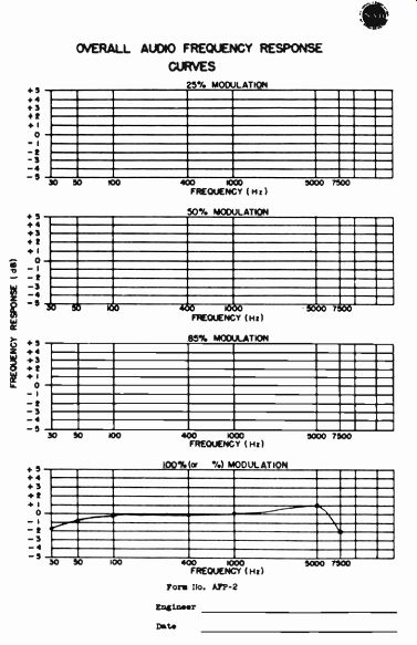
Fig. 14-15. Form for plotting frequency-response curves.
Noise Level
Hum and noise must be at least 45 dB below the level representing 100-percent modulation between 30 Hz and 20 kHz. The reference frequency is 1000 Hz, and this measurement may actually be performed in Step 5 of the preceding procedure by removing the oscillator (after the reference level has been established) and terminating the microphone-amplifier in put with a resistor equal to its input impedance. Leave all gains as originally set, but be sure that no other source faders are open. The noise-distortion meter is then placed in the noise mode and its sensitivity increased to obtain the noise level in the unmodulated carrier. The microphone input level should be no lower than -50 dBm.
The input tubes of preamplifiers are the most common cause of noise. If an oscilloscope is available, connect it to the scope terminals of the noise-distortion meter, and determine if the noise is caused by a hum component.
Many amplifier or preamplifier power supplies employ "hum" potentiometers which should be adjusted while the noise measurement is watched. Use the same trace-down procedure for hum and noise as that previously de scribed for running down the cause of an improper frequency response.
Audio-Frequency Harmonic Distortion
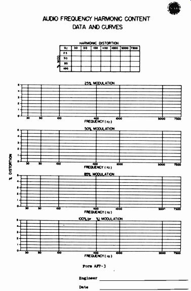
Fig. 14-16 illustrates the NAB-suggested
forms for recording the audio-
frequency harmonic content, which is normally measured in terms of percentage. The measurements must be taken at the modulation percentages indicated and at the specified single sine-wave frequencies. The noise-distortion meter must be capable of measuring throughout the harmonic spectrum required by the FCC. The harmonic distortion must not exceed 5 percent up to 84-percent modulation, or 7.5 percent for modulation percentages greater than 84 percent. A typical procedure for the measurement of audio-frequency harmonic distortion follows.
1. The reference modulation at the reference frequency (1000 Hz) is obtained as in the frequency-response procedure. The noise-distortion meter is then placed in the set-level position, and the meter is adjusted to 100-percent calibration.
2. The noise-distortion meter is then placed in the distortion position, and the tuning and bridge-balance controls are adjusted for minimum reading. The sensitivity is next increased in steps of 10 dB, and these controls are readjusted for minimum each time.
3. The percentage is read directly on the most sensitive scale possible to obtain a minimum reading by use of the tuning and balance controls.
Excessive harmonic distortion can be caused by tubes, low power-supply voltages, or overdrive of any amplifier or chain. Again, this is a case of tracing down the source of distortion first to the transmitter only, line or STL, or studio. Also, if excessive noise is present, the distortion measurement is apt to be high because of the noise level. It is important to keep the microphone input level from the audio oscillator no lower than -50 dBm.
Carrier Shift
Carrier shift is a change in the average value of the modulated rf carrier compared to the average value of the unmodulated carrier. A shift in the upward direction is called a positive carrier shift; a shift downward is a negative carrier shift. Excessive carrier shift results in unwanted harmonics and additional sideband frequencies with consequent interference on adjacent channels.
Fig. 14-17 illustrates a convenient form for use in recording the carrier shift data. A tone of 400 Hz is required. Assume, for example, that the rectified unmodulated carrier measures 1 volt. This is recorded in row 1.
Under modulation, the voltage drops to 0.95 volt. This is recorded under the first reading in row 2. The difference voltage is 0.05 volt, recorded in row 3. The ratio of the number in row 3 to the corresponding number in row 1 is 0.05/1, or 0.05. This is 5-percent carrier shift (negative) .
In practice, the rf input meter on the modulation monitor (which is normally adjusted to 100 percent in operation) may be used to measure this carrier shift. In the preceding example, if the modulated carrier exhibits a 5-percent negative carrier shift under modulation, the input meter will indicate 95 percent rather than 100 percent.
Courtesy National Association of Broadcasters
Fig. 14-16. Form for recording
harmonic-distortion data.
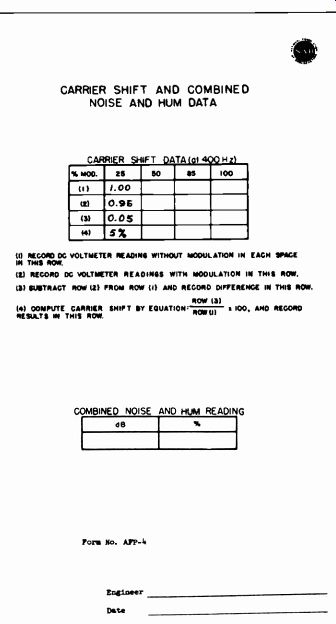
Fig. 14-17. Form for recording carrier-shift and noise and hum data.
The maximum carrier shift at any of the specified degrees of modulation must be less than 5 percent in either the positive or negative direction.
Excessive carrier shift may result from any of the following: overmodulation (check accuracy of modulation monitor with oscilloscope), improper grid bias, poor grid-bias supply regulation, poor plate-supply regulation, defective power-supply filters, faulty neutralization, or improper rf excitation
Spurious Radiations and RF Harmonics
Spurious radiations and rf harmonics must be kept at a minimum and must never be of sufficient amplitude to cause undue interference to other services. Fig. 14-18 is a suggested form for these measurements and is self explanatory.
Applicable FCC Rules (always check latest rulings) are as follows:
1. Any emission appearing on a frequency removed from the carrier by between 15 kHz and 30 kHz inclusive shall be attenuated at least 25 dB below the level of the unmodulated carrier.
2. Any emission appearing on a frequency removed from the carrier by more than 30 kHz and up to and including 75 kHz shall be attenuated at least 35 dB below the level of the unmodulated carrier.
3. Any emission appearing on a frequency removed from the carrier by more than 75 kHz shall be attenuated at least [43 + 10Logio (power, in watts)] dB below the level of the unmodulated carrier, or 80 dB, whichever is the lesser attenuation.
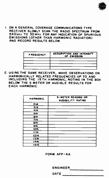
Fig. 14-18. Form for recording spurious-radiation and harmonic data.
(1) Record attenuator reading for the 1000-Hz reference signal in his row.
(2) Record the attenuator readings for the specified frequencies in this row.
(3) Record the AF response variations, which are obtained by subtracting row (2) from row (1), in this row. These final figures are to be used in plotting the graphs.
NOTE: The figures inserted in this example indicate pre-emphasis measurement.
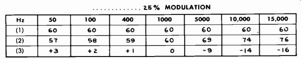
Fig.
14-19. Example of data from frequency-response check of fm transmitter.
14-7. PROOF OF PERFORMANCE (FM MONO)
The same technique as that previously described for AM is used for fm proof of performance; the essential difference is the broadened and more stringent requirements of performance. The frequency-response measurement may be taken either with or without de-emphasis. It is a good engineering practice to run this check both ways. This proves that the station de-emphasis network in the monitor circuit is essentially complementary to the 75-microsecond pre-emphasis.
Fig. 14-19 is an example of tabulated data obtained by measuring the transmitter output without de-emphasis. Just as in AM measurements, the entry in row 1 is the attenuator setting for the 1000-Hz reference frequency to obtain the specified modulation. Recorded in row 2 are the actual settings required at the specified frequencies to maintain the reference modulation. The numbers in row 3 are obtained by taking the difference between each entry in row 1 and the corresponding entry in row 2. Note: that as in the AM measurements the plus attenuator setting indicates that the response is lower. These figures are plotted on the standard 75-µs pre-emphases curve (Fig. 14-20) . Note in this example that the original run, where the 1000-Hz reference is 0 dB, results in the values for frequencies of 5000 Hz and 10,000 Hz falling outside the tolerable limits. Note, however, that at 5000 Hz (farthest out of the range) a shift of-0.8 dB brings this measurement within the limits. Therefore a new curve may be drawn (as shown by solid dots) with an axis shift of-0.8 dB, and the proof is satisfactorily completed. If this shift had resulted in other points falling outside the limits, remedial measures would have been needed to correct the fault. Measurements must be taken at least at the frequencies specified in Fig. 14-19 and for modulation percentages of approximately 25, 50, and 100 percent. The response is then run with standard de-emphasis, and the overall curve is drawn as shown in Fig. 14-15 for AM, except for the extended frequency range.
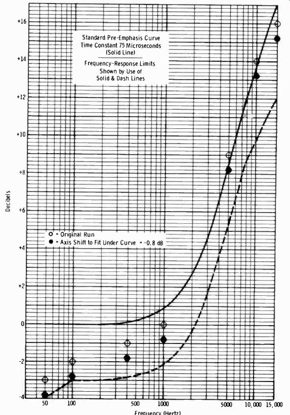
Fig. 14-20
......... allowable distortion (measured through a standard 75-1.ts de-emphasis circuit) is as follows:
50-100 Hz: 3.5 percent 100-7500 Hz: 2.5 percent 7500-15,000 Hz: 3.0 percent
The output noise level for fm is measured in two categories, fm noise and AM noise. The method of measuring fm noise is the same as that de scribed for AM in the preceding section. This includes any noise in the entire system that would result in frequency modulation of the carrier. Just as ir_ AM, fm noise is measured in dB below the level corresponding to 100-percent modulation, which for fm broadcast is a frequency swing of ±75 kHz. This measurement must be made with standard 75-us de-emphasis. The indicating instrument must have ballistic characteristics similar to those of a standard VU meter. The fm noise must be at least 60 dB below 100-percent modulation, with a 75-µs de-emphasis circuit employed.
It is necessary to obtain the AM noise level in terms of what would correspond to 100-percent amplitude modulation of the transmitter, but it is obviously not possible to amplitude modulate the fm transmitter to 100 percent. Some other means must be used to calibrate the noise meter.
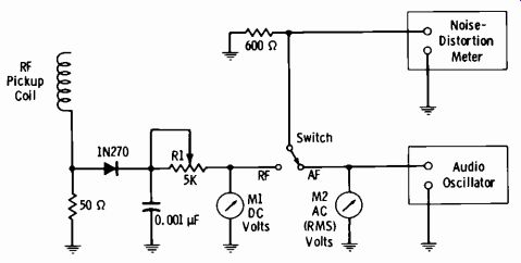
Fig. 14-21. One method of measuring AM noise level of fm transmitter.
The arrangement shown in Fig. 14-21 may be used for this purpose. A diode rectifier rectifies a small amount of rf energy from the output of the transmitter. A dc voltage proportional to the carrier output of the transmitter appears across the 600-ohm resistor with the switch in the rf position. Should the carrier output be amplitude modulated, there would also appear an ac voltage that would be proportional to the percentage of modulation. If the carrier were amplitude modulated 100 percent, this ac voltage (rms) would be equal to 0.707 times the dc voltage. (The rectifier is a peak-voltage rectifier.) Thus an external calibration of the noise meter can be set up. This is done with an audio oscillator having a 600-ohm output adjusted so that there appears across the output an ac voltage equal to 0.707 times the rectified dc voltage. This voltage is fed into the noise meter, and the latter is adjusted for full-scale deflection. Thus calibrated, it is ready for use in measuring the AM modulation level that appears across the output of the diode rectifier. The actual steps follow.
1. A diode rectifier is coupled to the output of the transmitter (Fig. 14-21) . In some transmitters, one-half of the audio-monitor coupling links may be used. Adjust R1 to obtain a convenient reading, such as 1 volt, on M1.
2. With the switch in the rf position, measure the dc output voltage of the diode rectifier by means of voltmeter M1.
3. Throw the switch to the of position, and adjust the output of the audio oscillator so that voltmeter M2 indicates an ac voltage equal to 0.707 times the dc voltage just measured. The noise meter is then adjusted to zero dB. (The reference is now set.)
4. Return the switch to the rf position, and read the noise level indicated by the noise meter. This is the measurement of the a-m noise level.
This level must be at least 50 dB below 100-percent modulation, with a 75-µs de-emphasis circuit employed.
Fig. 14-22 illustrates an alternate method of measuring AM noise with out the conversion factor of 0.707 described previously. Only one voltmeter is required. The procedure is as follows:
1. Open S2 and close S1. Adjust the trimmer capacitor (if used) and R1 to obtain a convenient voltmeter reading, for example 2 volts.
2. Open S1 and close S2. Adjust R2 to obtain exactly the same voltage.
3. Calibrate the noise meter for 0 dB reference.
4. Open S2 and close S1. Take the noise reading according to the instructions for using the noise-distortion meter.
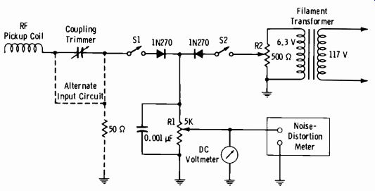
Fig. 14-22. Alternate method of measuring AM noise level of fm transmitter.
Spurious emissions are measured essentially as previously outlined for AM transmitters. The results must be as shown in Table 14-1.
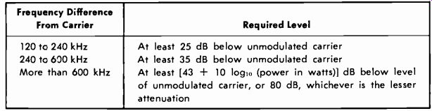
Table 14-1. Spurious-Emission Limitations (FM)
Frequency Difference
From Carrier Required Level 120 to 240 kHz 240 to 600 kHz
More than 600 kHz
At least 25 dB below unmodulated carrier
At least 35 dB below unmodulated carrier
At least [43 + 10 log10 (power in watts)] dB below level of unmodulated carrier, or 80 dB, whichever is the lesser attenuation
14-8. PROOF OF PERFORMANCE, MULTIPLEXED TRANSMITTERS (SCA & STEREO)
The basic principles of SCA and compatible stereo have been covered in previous Sections. This section is concerned with engineering standards, transmitter adjustments, and proof-of-performance measurements.
Engineering Standards for Subsidiary Communications Multiplex Operations
The following standards for SCA operation by fm stations are from paragraph 73.319 of the FCC Rules and Regulations.
A. Frequency modulation of SCA subcarriers shall be used.
B. The instantaneous frequency of SCA subcarriers shall at all times be within the range of 20 to 75 kHz, provided, however, that when the station is engaged in stereophonic broadcasting the instantaneous frequency of SCA subcarriers shall at all times be within the range 53 to 75 kHz.
C. The arithmetic sum pf the modulation of the main carrier by SCA subcarriers shall not exceed 30 percent, provided, however, that when the station is engaged in stereophonic broadcasting the arithmetic sum of the modulation of the main carrier by the SCA subcarriers shall not exceed 10 percent.
D. The total modulation of the main carrier, including SCA subcarriers, shall meet the requirements of 73.268 (85 to 100 percent modulation total).
E. Frequency modulation of the main carrier caused by the SCA subcarrier operation shall, in the frequency range 50 to 15,000 Hz, be at least 60 dB below 100 percent modulation, provided, however, that when the station is engaged in stereophonic broadcasting, frequency modulation of the main carrier by the SCA subcarrier operation shall, in the frequency range 50 to 53,000 Hz, be at least 60 dB below 100 percent modulation.
Measuring Cross Talk
The following is the RCA in-plant procedure for testing transmitters employing subchannel SCA before shipment. It appears here through the courtesy of RCA.
The measurement of special multiplex parameters should begin with main-to-subchannel cross talk. To set the reference, the subchannel should be modulated 100 percent (±7.5 kHz deviation) with a 400-Hz tone. Set the distortion analyzer for noise measurement, and adjust the meter deflection to 0 dB. The filter is set to pass a band of frequencies from 50 to 15,000 Hz (Fig. 14-23) .
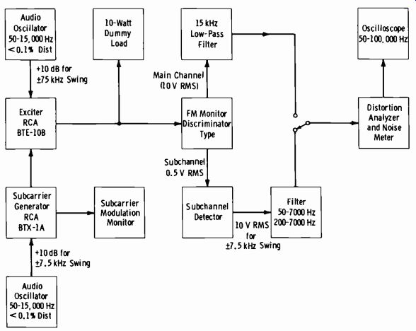
Fig. 14-23. Test setup for checking exciter and subcarrier-generator performance.
Now remove the subcarrier modulation and apply modulation to the main channel using several frequencies ranging from 50 to 15,000 Hz.
Adjust each frequency to 85-percent modulation if one subchannel is used.
(If two subchannels are used, the main channel should be modulated 70 percent instead.) Read the cross talk for every frequency on the distortion analyzer.
Next, modulate the main channel again with 400 Hz at 85 percent, and carefully adjust all multiplier stages of the exciter to give a minimum cross talk reading. Be sure not to detune the tuned circuits too much. Also touch up the monitor tuning (rf and IF coils and discriminator) , and be sure that the monitor and separate subcarrier adapter, if they are used, are fed with the right amplitudes and are not overdriven.
If it is necessary, repeat the steps previously indicated; however, a slight adjustment of the first tripler coil should correct any excessive cross talk on 67 kHz. By observing the waveform oscilloscope, make sure that the meter indication of the distortion analyzer represents the components required.
Certain beat frequencies generated in the monitor may give a false impression. It should be noted that the above adjustment is greatly simplified because only three tuned circuits may contribute to cross talk. In some in stances, it may be advantageous to shift the modulator grid-tuning capacitor slightly to give 2 to 3 dB better cross-talk reduction. The subcarrier modulator itself requires no tuning (in the RCA system).
Sub-to-main channel cross talk is measured in a similar way. This time the 0-dB reference is 100 percent modulation (±75 kHz deviation) by a 400-Hz tone on the main channel. This modulation then is removed, and tones from 50 to 6000 Hz are applied to the subcarrier generator, giving 100 percent (±7.5 kHz) modulation on the subchannel. Slight cross talk may result from improper balancing of the main-channel modulator tubes.
Therefore, the modulator-grid tuning, after an initial setting for maximum swing, should ultimately be tuned for minimum sub-to-main channel cross talk. This setting requires only a very slight change. The exciter multiplier tuning has practically no effect on sub-to-main channel cross talk.
To measure inter-subcarrier cross talk, one proceeds in the same way, set ting a reference level for the channel in which cross talk is being measured by first modulating it with a 400-Hz tone at 100 percent modulation (±7.5 kHz).
The cross talk measurement for the stereo subchannel is made by the same procedure as before, except that the main channel is modulated 90 percent instead of 100 percent (81 percent if SCA is included with stereo operation). The subchannel is amplitude modulated, and the suppressed-carrier sidebands frequency modulate the main channel.
To check the requirement in FCC paragraph 73.322(c), a "standard stereo receiver" or a reliable station receiving-type stereo monitor may be used. However, it is also possible to check the subcarrier generator itself.
An oscilloscope connected to a suitable point in the adder stage (addition of 38-kHz subchannel and 19-kHz pilot) may be used. The scope must have dual-beam provisions. The procedure is as follows:
1. Connect one scope input to the 19-kHz grid of the adder stage and the other input to the 38-kHz grid.
2. Be sure that no modulation occurs (no audio signal) .
3. Since the adder follows the balanced modulator, it is necessary (in order to obtain the 38-kHz subcarrier) to unbalance this circuit. This has no effect on the measurement.
(A) Subcarrier and pilot subcarrier.
(B) Proper detected main-channel output.
(C) Detected main-channel output in which L-R sidebands lag L + R.
(D) Detected main-channel output where L-R channel lacks sufficient gain.
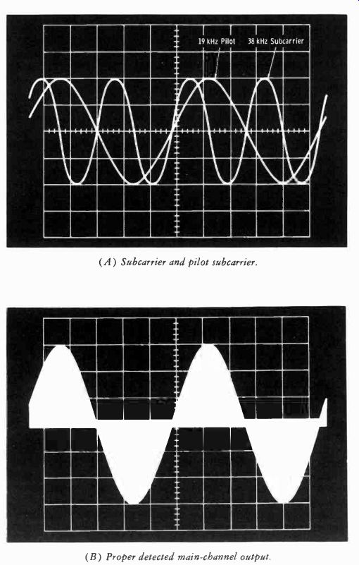
Fig. 14-24. Stereo waveforms.
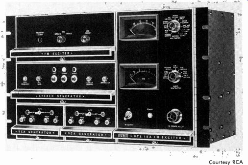
Fig. 14-25. RCA BTE 15A fm exciter.
4. See Fig. 14-24A. Note that each time the pilot crosses the zero axis, the subcarrier, which is the second harmonic of the pilot, crosses the zero axis in the positive direction.
The detector output waveform from the receiver should appear as in Fig. 14-24B. The waveform is a composite of the L + R signal and the L-R sideband signal for a 400-Hz left-only input signal. The zero axis should be straight for all modulating frequencies.
Fig. 14-24C indicates that although the amplitudes of L + R and L-R are correct, the L-R sidebands lag L + R. In this particular case the lag is 6°, which is twice that allowed by the FCC. If the tilt is in the opposite direction, the L-R sidebands lead the L + R signal. In general, the phase is within the 3° tolerance if the amplitude of either half of the waveform is 9 times the measurable height of tilt. Thus, if the scope gain is adjusted to allow 4.5 cm of deflection for half of the waveform, the tilt amplitude should be no more than 0.5 cm.
An improper amplitude ( insufficient gain) of the L-R sideband signal is indicated by the waveform of Fig. 14-24D. The phase is correct. If the bottom trace bowed upward instead of dipping, excessive gain of the L-R sideband signal would be indicated.
All stereo transmitters are accompanied by detailed instructions, and the maintenance engineer is obligated to become thoroughly familiar with the necessary adjustments of his particular installation to bring it within FCC specifications on proof runs. These procedures naturally vary according to the circuitry.
For example, the BTE 10B exciter in the above example is a tube-type unit (of which many are still in use) requiring more adjustments than the more recent RCA type BTE 15A all solid-state unit (Fig. 14-25) .
Modulation of the temperature-compensated basic on-frequency oscillator is achieved by applying the composite stereo or SCA signals from the BTS 1B and BTX 1B generators, respectively, to a pair of push-pull varicap diodes which are coupled to the frequency-determining resonant circuit of the basic oscillator. The output of the basic oscillator is isolated from the following buffer amplifier by a 10-dB resistive attenuator. Thus, the stability and modulation characteristics of the basic direct fm oscillator are not disturbed by following rf power amplifiers.
The output of the buffer amplifier, approximately 500 mW, is used to drive the 15-Watt, three-stage rf amplifier as well as the binary divider chain in the afc circuit. The basic oscillator, buffer amplifier, and afc circuit are mounted inside a shielded enclosure. The rf power amplifier is also completely shielded.
Automatic frequency control (afc) for the on-frequency basic oscillator is achieved by taking a sample of the buffer output and applying it to a chain of 14 divide-by-two frequency dividers. A low-frequency reference crystal operating at 1/1024 of the desired output frequency has its frequency divided by 16 in a binary chain. Integrated circuits operating in the saturated mode are used in both binary dividing chains. The outputs from the reference and basic-oscillator binary dividers are phase compared in a time-sharing IC comparator. The output of the circuit, which represents the afc error voltage, is filtered and applied to another pair of varicap diodes coupled to the basic-oscillator tuned circuit. Thus, the basic oscillator is phase locked to the 1024th harmonic of the oven-controlled reference crystal.
An off-frequency detector is incorporated in the design of the BTE 15A fm exciter. When the basic oscillator frequency is not phase locked to the reference crystal, an ac component appears in the afc output. This voltage is rectified to operate a relay the contacts of which can be used to turn off the fm transmitter.
Two multimeters are located on the hinged door in front of the regulated power supply section. One of these meters is used to indicate power supply and operating voltages within the exciter and 15-watt rf amplifier.
The second meter is a peak-reading voltmeter that is used to indicate key modulating signals.
The rf power output of the BTE 15A can be continuously adjusted from 7 to 15 watts by means of a front-panel control. The primary power is turned on with a circuit breaker. The rf output is turned on with a front-panel switch or by jumping contacts available on the rear of the unit. The exciter will tolerate load mismatches from short circuit to open circuit without damage to the output transistor. Another safety feature prevents turning on the 41-kHz SCA subcarrier when the stereo generator is in the stereo mode.
In the Model BTS 1B stereo generator, the left and right input channels are identical, each having resistive input terminations, isolating transformers, 15-kHz low-pass filters, and an operational amplifier for obtaining pre-emphasis. The pre-emphasis is convertible from 75 to 50 microseconds in the field, or can be removed entirely. The left and right channels can be matched to within I/2 percent gain difference and I/2° phase difference from 30 to 15,000 Hz, including the 15-kHz low-pass filters. These filters are less than 0.5 dB down at 15 kHz, and more than 50 dB down at 19 kHz and above. This insures an absolute minimum of disturbance to the pilot carrier and subcarrier regions by the program material.
The pre-emphasized and filtered left and right audio signals are applied to a switching modulator which alternately switches between the two audio channels. The balanced and symmetrical 38-kHz switching signal is de rived from a buffered 38-kHz output of a bistable multivibrator. The negligible amount of second harmonic (76 kHz) in the 38-kHz switching signal assures a minimum of interference to a 67-kHz SCA channel. The 76 kHz crystal-controlled signal driving the binary divider assures a frequency stable 38-kHz stereo subcarrier.
The output of the switching modulator, along with the sinusoidal pilot (less than 1 percent distortion), is applied to a phase-linear filter to remove the third and all higher-order harmonic components of the switching signal. The complete composite stereo signal, or a left or right monaural signal, is selected by relays and applied to the input of an operational amplifier. The output of this amplifier is then applied to the wideband input of the BTE 15A fm exciter.
Switching between monaural right, monaural left, or stereo may be accomplished by front-panel push buttons on the BTS 1B or by momentary remote-control contact closures. The selected mode is indicated by front-panel lamps. Left, right, and composite program outputs are also applied to a peak-reading meter on the main frame of the fm exciter.
The Model BTX 1B SCA generator, using all hermetically sealed metal-cased integrated circuits and transistors, is designed to operate on either the 41-kHz or 67-kHz SCA channels. The audio input is applied to a resistive terminating pad and then to an isolating transformer before being amplified. An optional 5-kHz low-pass filter may be inserted in the input to pre vent higher-order lower sidebands of the 67-kHz subcarrier from penetrating the upper regions of the stereophonic spectrum.
The audio amplifier includes an active pre-emphasis network which may be easily changed from 75 microseconds to 50 or 150 microseconds or adjusted for a flat response. The audio sensitivity of the BTX 1B is sufficiently high that line amplifiers are not required.
The processed audio input signal is then applied as modulation to a direct-fm SCA generator that includes a temperature-compensating circuit for extreme frequency stability. A vernier center-frequency control is avail able on the front panel.
Following this generator are a series diode muting gate, a buffer amplifier, and a wideband low-pass filter to remove subcarrier harmonics. The total harmonic content of the subcarrier output is less than 1 percent, and the incidental AM is less than 5 percent peak with 10 percent subcarrier modulation. The output of the low-pass filter is applied to another buffer amplifier and output level control for application to the multiplex input of the BTE 15A fm exciter.
A sample of the pre-emphasized audio is used to drive a peak-reading multimeter on the main frame of the exciter. Automatic muting of the subcarrier is accomplished in the following manner. A portion of the pre-emphasized audio is applied to a variable-gain amplifier and, with an adjustable time constant, peak detected to operate a Schmitt trigger circuit.
The output of the Schmitt trigger is shaped with a low-pass filter and used to turn on or off the series diode muting gate. When audio is applied to the input of the BTX 1B, the muting diode gate is turned on to allow the subcarrier output to appear. In the absence of audio, the Schmitt trigger pauses for a selected time interval before turning off the diode muting gate.
The subcarrier envelope rise and fall times are constant and so chosen as to minimize clicks and pops in an SCA multiplex receiver. The amount of Schmitt-trigger delay is adjustable with a front-panel control. With this control, subcarrier muting can be adjusted to occur from 0.5 to 5 seconds after the audio input is removed. Two transistors are used to operate front-panel lamps to indicate the on-off status of the subcarrier. Also, a front-panel switch provides manual control of the subcarrier output or the use of the automatic muting feature. The subcarrier also can be turned on or off remotely.
Stereo Adjustments and Proof of Performance
Fig. 14-26 presents a suggested setup at the studio for stereo proof-of-performance measurements. The audio generator, step attenuator, and VU meter are usually incorporated in one unit. The balanced Y pad splits the common audio signal into two paths for simultaneous left and right channel (microphone input) feeds. Switches S1 and S2 allow either left only, right only, or left plus right feeds. Switch S3 allows either normal or re verse polarity feed to the right-channel input. Note that in the normal position, the A output of the signal generator feeds terminals 1 and 3 of the input transformers, while the B output feeds terminals 2 and 4. Thus the two inputs are being fed with a common in-phase signal, where L = R.
With S3 in the reverse position, the polarity of feed to the right channel input is 180° out of phase with the left channel input, or L =-R. This is necessary for certain adjustments and measurements as described later.
When only the transmitter is to be tested to prepare for overall proof-of-performance measurements, the left and right inputs are to the inputs of the stereo generator. A typical setup at the transmitter for overall proof-of-performance runs is illustrated in Fig. 14-27.
Audio frequency-response and noise-distortion measurements are taken exactly as outlined earlier for mono fm, except that the procedure is repeated for the opposite channel. This simply means that the left and right channels must individually meet requirements of the FCC for the various modulation levels just as in mono fm specifications. We are then ready to take the remaining measurements which have to do with the composite signal: separation and cross talk between channels.
Left & Right
Input Channels
1 tMic Inputs)
Left In Right In
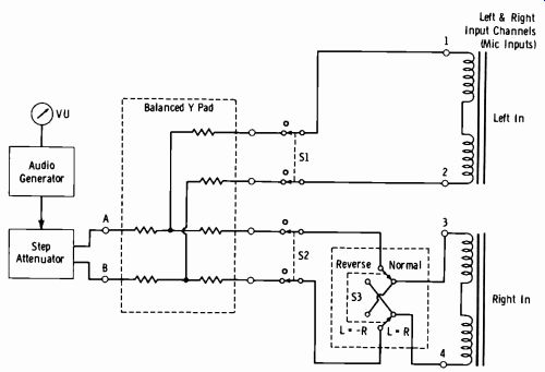
Fig. 14-26. Studio setup for stereo measurements.
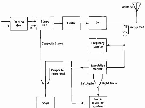
Fig. 14-27. Transmitter setup for stereo measurements.
The following is an outline of a typical preliminary adjustment procedure in preparing for stereo proof-of-performance runs. It is assumed that the signal generator is at the transmitter.
STEP 1: Connect the oscilloscope vertical input to the composite-signal output of the stereo generator. Sync the scope internally. Apply a left-only signal of 400 Hz at the specified input level of the stereo generator. Turn the pilot amplitude control to minimum.
STEP 2: The pattern on the scope should be as in Fig. 14-28A. If the base line is not flat (Fig. 14-28B) , adjust the left-channel (L + R) gain control (sometimes termed "separation" control) to obtain a flat base line.
STEP 3: Apply a right-only 400-Hz signal and repeat the above adjustment for the right-channel gain control. Sometimes both controls are used; sometimes only an L + R gain control is incorporated. The point is that when the two gains are equal, the base line will be flat.
CAUTION: When a sampling type of modulator is used, a large number of odd-order harmonics (3rd, 5th, etc.) of the 38-kHz switching rate exist. For this reason, an output filter is employed to confine component frequencies below 75 kHz. Sometimes an output-filter phase-linearity control is incorporated to set the driving impedance of the filter for maximum phase-shift linearity over the range of 50 Hz to 53 kHz. Misadjustment of this control will cause a left-only or right-only signal to appear very similar to the waveform of Fig. 14-28B. If it is not possible to obtain a perfectly flat base line by adjusting the L + R and/or L-R gains, investigate this possibility. More recent solid-state stereo generators employing the sampling tye of modulation have fixed filtering networks that require no adjustment. The same problem can occur, of course, with a component change or failure within the filtering network.
(A) L R and L-R gains equal.
(B) L R and L-R gains unequal.
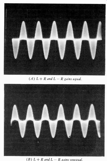
Fig. 14-28. Setting separation controls.
STEP 4: Reverse the polarity of the right-channel input (Fig. 14-26) , and feed both channels so that L = -R.
Turn the pilot amplitude control to normal. With the scope time base set at about 200 µs/cm, the pattern of Fig. 14-29A should be obtained. This is termed the L-R "butterfly" and can be used to adjust the pilot phase control accurately. Remember that proper phase is indicated when a zero crossing of the pilot signal occurs at precisely the same time as the positive-going zero crossing of the (sup pressed) 38-kHz subcarrier (Fig. 14-24A) .
STEP 5: Expand the time base of the scope to around 50 µs/cm. Trigger the scope externally with the signal-generator frequency or the 19-kHz pilot. If the pilot phase is correct, a perfect diamond pattern such as that of Fig. 14-29B will be displayed. This indicates proper zero crossings of the pilot and subcarrier sine waves. If the phase is not correct, the four crossings do not form a diamond pattern, and a distorted presentation such as that of Fig. 14-29C is obtained. Adjust the pilot phase control so that the pattern of Fig. 14-29B is obtained. Always recheck the pilot gain after pilot phase adjustments are made.
STEP 6: Move the scope to the modulation monitor position. The scope display from the composite output of the modulation monitor should be identical to that obtained from the composite output of the stereo genera tor. If a different pilot phase is indicated, adjust the pilot phase control in the monitor to agree with the phase shown at the composite output of the stereo generator, or follow specific instructions of the monitor manufacturer.
Measuring Separation
Feed a signal of 1 kHz to either the left or right (only) input. With the modulation monitor set in the Total position, modulate the transmitter 100 percent. Switch the modulation meter to the channel opposite that being fed; the modulation indication should be at least 29.7 dB below the 100-percent modulated channel (actually 90 percent with 10-percent pilot) .
This condition should prevail over a frequency range of 50 Hz to 15 kHz.
Measuring Cross Talk
The left and right input channels of the stereo generator are connected in parallel and in phase. The frequencies at which cross talk is to be measured modulate the main (L + R) channel without modulation of the subchannel (L- R) . With the main channel at 90-percent modulation (10-percent pilot modulation) , cross talk of the main channel into the sub-channel is then indicated on the modulation monitor in the L-R position.
The percent modulation in this channel should be a maximum of 1 percent, indicating -40 dB of cross talk.
Next, reverse the phase of the signal to the right channel, and set L-R to 90-percent modulation. Cross talk of the subchannel into the main channel is now indicated by the L + R position of the modulation monitor.
Problems in Stereo Proof of Performance
The problems of frequency response, fm and AM noise of the fm carrier, and distortion are no different from those previously described for the mono fm transmitter, except that the number of measurements is essentially doubled. As in mono fm, poor performance is isolated to transmitter only, lines or STL from studio to transmitter, or the studio.
The cross-talk specification is usually the most difficult to meet. This measurement should first be made on the transmitter alone to check adjustments of the stereo generator, exciter and power amplifiers, and antenna system. If the cross-talk measurement deteriorates between the stereo-generator output and the final-stage output, check for proper circuit tuning and stage neutralization.
After the stereo generator and following rf stages have been optimized, move the signal generator to the terminal gear where the STL or wire lines normally feed. Unequal phase shifts and/or gains through agc or limiting amplifiers can cause major cross-talk problems. Gain must be kept to within one percent and phase to within one degree if cross-talk specifications are to be met.
Next, the signal generator is moved to the input of the STL or lines at the studio. Thus any additional factors in this area will influence the measurements. The final step is to feed the left- and right-channel microphone in puts for the regular overall proof-of-performance measurements.
(A) Time base of 200 us/cm. (B) Time base of 50 us/cm, correct phase.
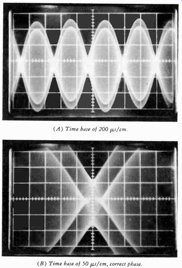
Fig. 14-29. L- R display to. setting pilot phase.
(C) Time base of 50 µs/ cm, incorrect phase.
14-9. PREVENTIVE-MAINTENANCE SCHEDULES
Of course, the primary purpose of any preventive-maintenance schedule is to reduce as much as possible the likelihood of a failure of any component part of the broadcasting installation during the broadcast day. Regular maintenance schedules are in effect at most broadcast stations and do much to increase the useful life of equipment and anticipate many tube and parts failures that would otherwise occur.
Preventive maintenance on any sort of equipment may be defined as a systematic series of operations performed periodically on the equipment in order to prevent breakdowns. This type of maintenance may be divided into two phases: work performed while the equipment is functioning, and work performed during the normal shutdown periods. This discussion is concerned only with preventive maintenance procedures carried out during the shutdown period.
The importance of preventive maintenance cannot be overestimated.
The owners of a broadcast station depend on its being on the air every second of its scheduled periods of transmission. It is very important that the personnel maintain the equipment so that lapses in the transmission will be kept to a minimum.
Cleanliness of the equipment is of the utmost importance since collections of dust and dirt can cause a number of troubles. This is particularly true in the higher-power stages of transmitters, since accumulation of foreign matter over a period of time reduces the effectiveness of the insulation to a point where leakage currents and arc-overs are common. High-voltage contacts have an extreme tendency to collect dirt (this is the principle used in electronic smoke eliminators), and the higher relative humidity existing in summer or in southern locations tends to aggravate this characteristic. A dusting and clean-up procedure, then, is desirable at a transmitter plant. A source of dry air under pressure is a common means of blowing out dirt, dead insects, and the like from inaccessible corners and from variable tuning capacitors. Insulators, safety gaps, etc., should be polished with a dry cloth. Carbon tetrachloride may be used to loosen excessive dirt and grime.
Transmitter Maintenance Schedule
So that preventive maintenance is effective, it must be performed at regular intervals; that is, certain portions of the equipment must be inspected for certain things every day in older-type equipment, while other parts of the equipment need be inspected only weekly or monthly. The following is a comprehensive maintenance schedule that may be considered a guide to anyone desiring to set up a means of preventing breakdowns. Naturally, this listing may include items that are unnecessary at a particular station, but it has been compiled with the thought that very precaution should be taken.
A. DAILY
1. Hourly read all meters and check power-tube filament voltages.
2. Check air-cooled anode temperatures. Check water temperature of water-cooled tubes if used.
3. Check for correct cabinet temperature of air around high-voltage rectifiers.
4. After shutdown, make a general inspection for overheated components, such as capacitors, inductors, transformers, relays, and blowers.
5. Investigate any peculiarities of meter readings.
6. In case of overloads, examine safety gaps and transmitter components for arc pits, etc. Clean and polish surfaces where arcs have occurred.
Reset gaps if necessary. Investigate causes of outages.
7. In the event of lightning or heavy static discharges, inspect the trans mission line, terminating equipment, and the antenna including the gaps. Polish pitted surfaces.
8. If gas-filled coaxial line is used, check pressure.
B. WEEKLY (In addition to items in daily inspection)
1. Immediately after shutdown, check antenna-terminating components for signs of overheating.
2. Clean antenna-tuning apparatus. Check for arc pits, etc. Clean and polish gaps and adjust if necessary.
3. Test antenna monitor rectifier tubes.
4. Calibrate remote antenna meters against meters at the antenna.
5. Clean transmitter using a vacuum cleaner.
6. Clean component parts of transmitter.
A. Brush terminal boards.
B. Clean insulators with carbon tetrachloride.
C. Clean power tubes and high-voltage rectifiers with tissue and alcohol or distilled water.
7. Check filament voltages and dc voltages at the sockets of all tubes that are not completely metered by panel meters.
8. Check air-flow interlocks for proper operation. Check all door interlocks for proper operation.
9. Check operation of grounding switches. Examine mechanical operation and electrical contacts.
10. Inspect blowers for loose impellers, free rotation, and sufficient oil.
11. Inspect relays for proper mechanical and electrical operation. If necessary, clean and adjust components.
12. Inspect air filters; clean if excessive dirt has accumulated.
13. Check all sphere and needle gaps. Clean any pits or dirt. Check gap spacings.
14. Check filter-bank surge resistors with an ohmmeter.
15. Check any power-tube series resistors with an ohmmeter.
16. Check power-change switches if used; check for serious arcing during day-night antenna changeover if used.
17. Make general performance checkup (distortion, noise, and frequency response) . Observe modulated waveform on cro.
18. Check neutralization by disabling crystal oscillator and observing grid currents.
19. Check proper operating voltage for pure-tungsten-filament tubes.
Determine lowest permissible voltage as follows:
A. AM transmitters-distortion and carrier-shift checks.
B. Fm transmitters-decrease filament voltage until output begins to drop.
C. Operate filaments approximately 1 percent above the filament voltage determined in A or B.
20. If water cooling is employed, check entire system for any signs of leakage and for electrical leakage.
21. Check pressure of any gas-filled capacitors.
C. MONTHLY
(In addition to daily and weekly items)
1. Make detailed inspection of all transmitter components using what ever tests seem advisable.
2. Clean and inspect tube-socket contacts and tube pins.
3. Clean or replace air filter. Brush dirt from blower impellers, canvas boots, etc.
4. Clean and adjust all relay contacts. Clean pole faces on contactors.
Replace badly worn contacts.
5. Oil the blower motors (carefully) .
6. Operate all spare vacuum tubes for a minimum of two hours under normal operating conditions. Clean up any gassy tubes as described in a later section on large power tubes.
7. Operate all spare mercury-vapor rectifiers normally, after first applying filament voltage only for a minimum of 30 minutes. Store the tubes upright.
8. Inspect all variable-inductor contacts for tension, signs of overheating, and dirt. Clean and adjust as required. Carbon tetrachloride or crocus cloth may be used for cleaning. Do not use emery cloth.
9. Check for proper operation of time delays, notching relays, and any automatic-control systems.
10. Clean audio-equipment (console, etc.) attenuator and low-level switching contacts with cleaner; wipe off excess.
11. Check tubes in station monitoring equipment, such as frequency monitor, modulation monitor, etc.
12. Clean switches in monitoring equipment with cleaner.
D. QUARTERLY
(In addition to the preceding)
1. Lubricate tuning motors and inspect for ease of rotation.
2. Check all indicating meters. Check ac filament voltmeters with an accurate dynamometer-type meter.
3. Check all connections and terminals for tightness.
4. Inspect any flexible cables to door connections.
5. Inspect and lubricate if necessary any flexible drive cables.
6. Inspect, clean, and service (if necessary) all switches (voltmeter selector switches, push-button switches, control switches, etc.) .
7. Clean transmission-line insulators, and take up slack if open-wire lines are used.
8. Check oil circuit breakers, if used, for sufficient oil and loose or defective parts.
E. SEMI-ANNUALLY (In addition to the preceding)
1. Test transformer oil for breakdown, and filter it if necessary. (This is done by the power company.)
2. Check protective overload relays or circuit breakers for correct operation.
A. Ac overload relays may be checked by shorting the high-voltage transformer secondary.
B. Dc overload relays may be checked by shorting the dc through the relay in the circuit protected by the relay.
3. In fm installations, check the accuracy of the modulation monitor as described below.
Measuring Frequency Deviation by the Bessel-Zero Method
An fm wave may be resolved into its carrier and sideband-frequency components, the amplitudes of which vary as Bessel functions of the modulation index. The modulation index is defined as the ratio of the peak deviation from the center frequency to the frequency of the modulating signal:
AF m=
where, m is the modulation index, OF is the peak deviation in Hz, f is the modulating frequency in Hz.
At certain values of m, the carrier amplitude becomes zero; that is, all the energy is transmitted in the sidebands. Fig. 14-30 shows relative carrier amplitude as a function of modulation index. Table 14-2 gives the modulation indexes necessary to produce successive carrier nulls. If the modulating frequency (f) is properly chosen, one of the carrier-null points can be made to correspond to the desired maximum deviation. For example, the peak deviation for an SCA subcarrier is ±7.5 kHz. For the first null, the modulating frequency (f) must be:
mF 7'5 Hz 3 125 kHz 2.4
Obviously, for the main carrier with a ¿F of ±75 kHz, the modulating frequency must be 31.25 kHz to use the first null. Since this modulating frequency is outside the passband of the audio system, the second null must be used, and the modulating frequency becomes f = 75 kHz/5.52 = 13.586 kHz, which is practical. However, the alternate method described later may be used.
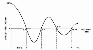
Fig. 14-30. Variation of carrier amplitude with modulation index.

Table 14-2. Modulation Indexes Required for Carrier Null