Signal generators have literally thousands of applications, and no book could attempt a complete discussion of all of them. However, in this section we include a few examples of what can be done with signal generators. With such examples in mind, the reader should have no difficulty in picturing many others, and of finding more and better ways of adapting these instruments to his own particular problems.
I. A-M RECEIVER ALIGNMENT
10-1. Review of A-M Receiver Alignment Procedure
The details of a-m receiver alignment procedures have been discussed and explained for many years in much of the available technical literature. It is suggested that for an exhaustive coverage of this subject the reader consult any good book on radio servicing. However, since a-m receiver alignment is one of the most commonly used applications of the a-m signal generator, let us review briefly the fundamental steps involved for the sake of completeness and for refreshing our memory.
A-m receiver alignment for standard broadcast receivers is reviewed in the table, which outlines the steps normally followed.
The table indicates in step 1 that the signal generator is connected to the grid of the mixer. This does not have to be a direct connection in most cases, but the generator can be as loosely coupled as is possible, consistent with a strong enough signal for alignment purposes. In the majority of set-ups, the connection can be through a small capacitor (50 u-u-f or less), or through a loop of wire placed over the mixer tube, as is done with many tv receivers. In fact, there is often no need for any connection at all, since radiation from the leads (and all too often directly from the generator when low-cost types are used) may provide sufficient signal in the i-f amplifier itself to satisfy all alignment requirements.
==========
ALIGNMENT PROCEDURE (For standard-band superheterodyne receivers)
Note: Check adjustments at the high-frequency end of the band after aligning the low-frequency end.
-------
Connect Signal Generator to:
1. Mixer grid (loose coupling)
2. Antenna terminals through dummy antenna •
3. Antenna terminals through dummy antenna •
4. Antenna terminals through dummy antenna •
---------
Set Signal Generator Frequency at:
Specified i.L
Specified oscillator high-frequency adjustment (usually 1400 khz)
Specified antenna high frequency adjustment
Specified oscillator low frequency adjustment (usually 600 khz)
-------------
Adjust Trimmers in Order Shown:
Output i-f transformer secondary, output i-f transformer primary, input i-f transformer secondary, input i-f transformer primary
Oscillator shunt
Mixer shunt, antenna shunt
Oscillator series or ganged capacitor plate
======================
The same is true of the injection of the signal into the antenna circuit, as called for in steps 2, 3, and 4. As explained in Section 7, a standard dummy antenna can be used to ensure that the load on the antenna circuit is proper for r-f circuit alignment. However, with so many a-m broadcast receivers using loop antennas, it is generally more convenient to connect the signal generator to a small coil of wire or another loop antenna and bring this coil or loop near the loop antenna of the receiver. This couples the signal without appreciable change in the actual load normally used on the antenna circuit.
It is assumed that the alignment steps in the table are performed by use of a modulated signal with an output meter as an indicator in the a-f output circuit, or with an unmodulated signal and a VTVM reading d-c voltage at the ave lead. All these adjustments are then for maximum reading. When the output meter is used, care must be used to avoid effects of overloading by the application of too much signal to the receiver.
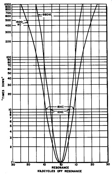
Fig. 10-1. Typical a-m broadcast receiver selectivity curves.
II. A-M RECEIVER PERFORMANCE TESTS
10-2. Selectivity
It has been previously pointed out that for accurate selectivity tests of a-m receivers, the signal generator must have an accurate step attenuator and some means of varying frequency accurately over a small range on either side of the center of the selectivity response checked. The latter facility can be provided by a vernier or fine tuning dial (see Section 5), or by a separate frequency meter or accurately calibrated receiver.
Selectivities are most commonly expressed in terms of "times down" of the output at a given bandwidth. In other words, a selectivity might be given as "bandwidth at 10 times down is 9 khz." The expression "times down" means that the voltage output of the receiver or receiver section being tested is that many times as small at the edges of the bandwidth stated as it is directly at resonance with a given received signal. Or, expressed differently, the expression is the ratio between the input off resonance to the input at resonance for a standard output. Typical selectivity curves are shown in Fig. 10-1, one for each end portion of the broadcast band. The selectivity is frequently greater (pass band smaller) at the low-frequency end (550 khz) because the r-f selectivity is greater there due to higher circuit Q's and adds to the i-f selectivity. As an example of the expression in words of the selectivity expressed by these curves, note that at 10 times down, the low-frequency bandwidth is about 12 khz and the high-frequency bandwidth is about 18 khz.
Both the arrangement of equipment and the procedure in taking selectivity measurements are shown in Fig. 10-2. First, in step (A), the generator is coupled to the receiver through a dummy antenna. Coupling may also be through a loop of wire coupled to the receiver's loop antenna, but in this case means must be taken to ensure that the coupling stays absolutely constant, since the amplitudes of the signals are important in this test. Another alternative in coupling is to insert the low impedance signal generator lead so the generator is in series with the low side of the loop antenna of the receiver. Then the step attenuator of the generator is set to the lowest setting possible for reasonable output from the output meter, with a modulated generator signal. In the figure it is assumed that the generator is started at the XI position of the attenuator switch. The signal used should be as weak as is consistent with a reason able output, to avoid overloading of the receiver. In some cases, it may be desirable to disable the ave. The adjustment of step (A) is made with the receiver carefully tuned to the generator signal so that the receiver is at exact resonance.
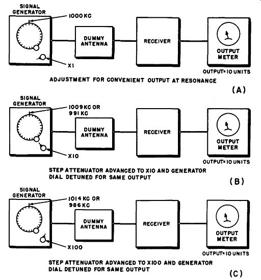
Fig. 10-2. Three steps in determining the selectivity of an a-m receiver.
ADJUSTMENT FOR CONVENIENT OUTPUT AT RESONANCE (A)
STEP ATTENUATOR ADVANCED TO X10 AND GENERATOR DIAL DE-TUNED FOR SAME OUTPUT (B)
STEP ATTENUATOR ADVANCED TO X100 AND GENERATOR DIAL DE-TUNED FOR SAME OUTPUT (C)
Proceeding to step (B), we turn the step attenuator to its X10 position (or the next higher position). The output naturally increases so the output meter reads much higher than before. Now, without touching any other controls, we detune the signal generator frequency from resonance until the output reduces to the same value as in step (A). When this has been done, we determine the actual new frequency of the generator. This is done either from a vernier or fine tuning dial on the generator, or by a separate frequency meter or calibrated receiver.
In step (C), we follow the same procedure, this time turning the step attenuator to X 100 without touching any other controls. The generator frequency is now further detuned until the output meter again reads the same as in step (A). Now the generator frequency is again determined.
The difference between the resonant frequency and that of step (B) multiplied by 2 is the bandwidth at "10 times down." The difference between the resonant frequency and that of step (C) multiplied by 2 is the bandwidth at "100 times down." For example, with the figures given in Fig. 10-2, the bandwidth at 10 times down is 18 khz and the bandwidth at 100 times down is 28 khz. Of course, the same procedure can be used for "1,000 times down", "10,000 times down", and to as high a ratio as desired.
If the response of the receiver is known to be quite symmetrical, readings on only one side of resonance are necessary, but otherwise it is safer to detune to each side of resonance in each case. When this is done, it is not necessary to multiply by 2 as mentioned above. As has been previously stated, the output can be observed just as well with an unmodulated signal input if the readings are taken with a vacuum-tube volt meter at the ave lead.
10-3. Sensitivity
For measurement of the sensitivity of a receiver, the signal generator must have an accurate indicator of generator output voltage. Sensitivity is expressed in terms of the signal voltage that must be applied to the input terminals (antenna terminals) of the receiver to produce a specified output power at the loudspeaker circuit. The receiver output power is measured either with the loudspeaker or a dummy load connected to the voice coil secondary winding of the output transformer.
The arrangement of equipment for sensitivity tests is shown in block diagram form in Fig. 10-3 (A). At (B) is shown the connection of the dummy load in the output circuit and the connection of an a-c meter to read the audio voltage across it. As in the selectivity test, the signal generator may be coupled either through a dummy antenna, as shown here, or through another type of coupling device. However, in this test, if the generator is not connected directly through a dummy antenna or in series with the low side of the loop antenna, the voltage-transfer characteristics of the coupling device must be known, so the sensitivity in microvolts will be correct.
The procedure in determining sensitivity is as follows: First, a weak signal from the signal generator is tuned in on the receiver, with the carrier frequency at the value at which the sensitivity reading is desired.
The output power is then observed, by reading the voltmeter or output power meter at the loudspeaker circuit. The signal generator output voltage is then changed until the output power is the specified value.
Standard output meters which read directly in power output, and are adjustable for various load resistance values, are available for this purpose. Otherwise, a non-inductive load resistor R, of the same resistance as the impedance of the loudspeaker voice coil, may be used, and the output power calculated from the voltage across it. In the latter case, the specified standard power output at which the sensitivity is to be measured is used in the formula:
E=-__/PR to determine the desired voltmeter reading. Adjustments are then made at the signal generator until the specified power output is indicated. The receiver tuning should be checked periodically to make sure the receiver remains at resonance with the generator signal.
When the receiver has been kept in exact resonance with the generator signal, and the generator output voltage has been adjusted for the minimum value at which full specified output power can be obtained, the output voltage of the generator is the sensitivity. Ordinarily, sensitivity is measured with the receivers volume control advanced to maximum.
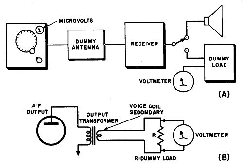
Fig. 10-3. (A) Equipment set-up for sensitivity tests. (B) Method of output
voltage indication.
Standard output is normally 500 milliwatts for high-output receivers (1 watt or more), and 50 milliwatts for low-output receivers. In either case, the output power and condition of controls of the receiver should be specified. Standards also call for a signal generator modulation frequency of 400 hz and a modulation percentage of 30 percent for this test.
The sensitivity may be expressed in microvolts, or in db below 1 volt.
For example, if the sensitivity is 100 microvolts, this is one ten-thousandth of 1 volt. A voltage ratio of 10,000 is equivalent to 80 db; thus the sensitivity of 100 microvolts can also be expressed as 80 db below 1 volt.
10-4. Signal-to-Noise Sensitivity
The sensitivity as determined in Section 10-3 is quite adequate for ordinary a-m broadcast receivers and other receivers in which the random noise is negligible. However, in short-wave and all-wave receivers, and very sensitive a-m broadcast receivers, random noise may become appreciable when weak signals are being received. It is therefore of special interest to know at how weak an input signal both the specified output power and the specified signal-to-noise ratio can be maintained.
The set-up for doing this is the same as in Fig. 10-3. Now, however, there is an extra step. The modulation of the generator signal is shut off but the carrier is left on; just the random noise in the presence of the carrier will then register on the output meter, and this indication is noted. Then the modulation is turned on and the output power checked.
The attenuators of the signal generator and the receiver controls must then be juggled back and forth until the output with modulation is the specified standard value (50 to 500 mw) and at the same time is greater than the noise level without modulation by the proper specified amount.
A typical signal-to-noise specification is 20 db, that is, modulation output voltage is 10 times the noise output voltage.
10-5. Overall Frequency Response
Overall frequency response is a check of how the output a-f modulation voltage at the loudspeaker terminals varies with variation of the frequency of the modulation, with modulation percentage and carrier strength constant. It is a check on the combined effects of r-f selectivity, i-f selectivity, and a-f amplifier response. It is sometimes referred to as a "fidelity" test, but this term is not too accurate since the test is of frequency response only, and there are many other factors involved in true fidelity.
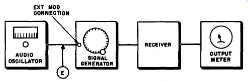
Fig. 10-4. Block diagram of set-up for checking overall receiver frequency
response.
The arrangement of equipment is shown in Fig. 10-4. The signal generator must have a connection for applying modulation from an external source. A suitable external source in this case is an audio oscillator, which is fed into the signal generator to modulate the carrier.
The modulation of the signal generator carrier can then be varied as desired. As a check on the modulation percentage, which must be kept constant during the test, the a-f voltage from the audio oscillator should be measured at E. When the set-up is ready, the audio oscillator is set for 400 hz.
The signal generator and receiver controls are then adjusted for a moderate output voltage indication. Then the audio oscillator is set successively for various values of audio frequency, and the output voltage for each noted. The voltage E is kept constant by adjusting the attenuator on the audio oscillator whenever E varies from its original value. E must of course be an a-c meter, to read the audio voltage. Except for an occasional check of receiver tuning to keep it at resonance, the other controls should not be touched during a frequency run.
Typical overall response curves are shown in Fig. 10-5. If the receiver has a tone control, it is of interest to note its effect by plotting one curve with each tone control position, as has been done here.
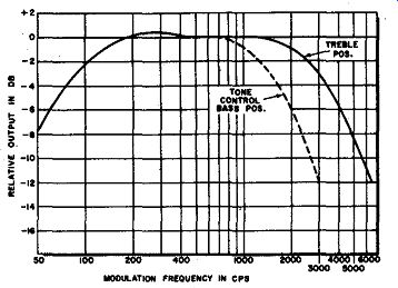
Fig. 10-5. Typical overall frequency response curve, for a-m broadcast receiver.
The tone control in this case is the simple type most frequently used in moderately
priced receivers. As can be seen, it provide, "bass," by reducing
the high-frequency component, of the modulation signal in relation to the lows.
10-6. Gain Measurements
The gain of a receiver stage or section is the ratio of output voltage to input voltage. There are several ways this gain can be measured using a signal generator. The main problem involved is that, in r-f and i-f sections, the measuring instrument and signal generator tend to load or detune the circuits.
The simplest and most direct method is to introduce a signal into the receiver, then measure the input and output voltages of the stage with a high-frequency probe connected to a vacuum-tube voltmeter. The accuracy depends upon how small the loading and detuning effects of the probe are, and these of course increase with frequency. Quite accurate results can be obtained in an i-f amplifier operating at 455 khz, whereas at tv intermediate frequencies and those of f-m broadcast receivers, results at best are only approximate.
Fig. 10-6. Typical arrangement far measuring stage gain.
Another even greater difficulty arises with this direct method. That is the fact that there are not many meters with scale ranges low enough to measure the input and output voltages of any but the output i-f amplifier stages. For this reason, it is considered preferable to move the signal generator connection point instead of the measuring device.
The set-up for this is shown in Fig. 10-6. The generator is first connected through a suitable matching and isolating circuit to point 1. The generator output voltage is adjusted for a convenient output voltage on the output meter, making· sure the signal is low enough to avoid over loading effects. To operate the output meter, the generator signal must be modulated at a constant percentage. The signal generator output voltage indication is noted. Then the signal generator lead is moved to point 2. The signal generator attenuator is now readjusted until the signal generator voltage rises enough to provide the same output voltage as before. The ratio of the two signal generator output voltages is the gain of the stage. For example, if it takes 100 microvolts at point 1, and 10,000 microvolts at point 2 to provide the same output reading in the loudspeaker circuit, the gain of the stage is 10,000 divided by 100, or 100.
III. SOME GENERAL A-M SIGNAL GENERATOR APPLICATIONS
10-7. Use as a Beat Frequency Oscillator for C-W Reception
Many short-wave and all wave receivers provide good reception on the short waves for radiotelephone stations, but do not contain a beat oscillator for code (c-w) reception. For such reception, a tone should be heard whenever the key is down at the transmitting station, and should stop when the key is up. This helps to distinguish dashes and dots and thus makes the code more readable. Without a tone, merely a series of clicks are heard.
A signal generator can easily be used to provide a beat oscillator for a receiver. Determine the intermediate frequency of the receiver; this will normally be within the tuning range of nearly all regular a-m signal generators, being most frequently 455 khz or near it. Next couple the generator loosely to the antenna circuit of the receiver, or by means of a loop of wire around the mixer tube if the latter is glass. If not enough input is obtained at the antenna circuit, the mixer-tube loop may be necessary. If the mixer tube is metal and therefore shielded to prevent the generator signal from getting in, couple the generator by means of a small piece of insulated wire, one end of which is connected to the generator hot output lead and the other end shoved under the chassis near the i-f amplifier tube.
After both receiver and signal generator have warmed up, tune in a signal on the receiver. With this signal being heard, tune the signal generator through the intermediate frequency; as it approaches that frequency, a beat note should be heard from the receiver. This beat note will start at a very high pitch and become lower in pitch as the inter mediate frequency is approached. When the signal generator signal is at the intermediate frequency the beat note falls to zero. Further adjustment of the generator frequency in the same direction results in a rise in beat-note frequency until it disappears. For receiving c-w signals, simply adjust the generator frequency for desired pitch of beat signal.
The same effect can be produced by tuning the signal generator frequency to the carrier frequency of the received signal, but this requires that the generator frequency be readjusted each time the receiver is tuned to a station of different frequency. This is not necessary when the generator is tuned to the receiver's intermediate frequency.
10-8. Substituting for the Receiver local Oscillator
In some short-wave receivers, the highest frequency bands tend to be unstable, with frequency drift and "jumpiness" of tuning. If a good stable signal generator is available, this condition can be remedied by using the signal generator output for the local oscillator signal. The signal generator is simply coupled to the oscillator grid or the signal grid of the converter or mixer tube, and the oscillator tuned circuit is shorted out, as shown in Fig. 10-7.
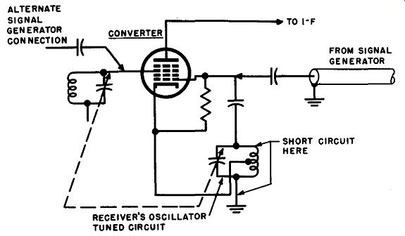
Fig. 10-7. Methods of injecting the signal generator output voltage into a
receiver circuit so as to substitute for the receiver's local oscillator.
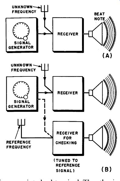
Fig. 10-8. Two ways of using a signal generator for frequency measurement.
Tuning is then by means of the signal generator dial, with the receiver dial used as a "trimmer" to be tuned for maximum reception on each station. The signal generator attenuator can be adjusted for optimum injection voltage. The frequency of reception is then the signal generator frequency plus or minus the intermediate frequency, the plus or minus depending upon which the receiver dial is tuned to.
10-9. Using a Signal Generator as a Frequency Meter
The simplest way to use a signal generator as a frequency meter 1s to feed the signal from it into the receiver along with the signal whose frequency is to be determined. Then the signal generator is tuned until its signal zero beats the signal of unknown frequency. The signal generator frequency is then the same as that of the unknown signal, and, if the signal generator dial is accurately calibrated it will indicate the desired frequency. This set-up is illustrated in Fig. 10-8 (A). Unfortunately, because of the large range of frequencies most a-m signal generators must cover, their dial calibrations are not such as to give a very close frequency reading. The signal generator is thus more useful as a frequency standard. In this application, the signal generator is tuned to some fixed low reference frequency, and its harmonics form "markers" through the frequency spectrum to the range in which the frequency to be measured is located. For example, if the generator is tuned to exactly 100 khz, there will be harmonics at 200 khz, 300 khz, etc.
In the a-m broadcast band there will be harmonics at 600 khz, 700 khz, 800 khz, etc.; at 20 mhz there will be one at 20 mhz, 20.1 mhz, 20.2 mhz, 20.3 mhz, and so on, at every tenth of a mega-cycle. The accuracy of each harmonic is the same in percentage as that of the original 100 -khz fundamental. With all these harmonics present, their exact locations on the dial of the receiver can be noted. There will be a 100 -khz harmonic on each side of the unknown signal. The latter's frequency can then be interpolated by its relative Position between them. The set-up is shown in Fig. 10-8 (B). If there is difficulty in determining which 100-khz harmonic is which, the signal generator may be switched to 1,000 khz, to produce harmonics every 1,000 khz (every megacycle). The nearest mega cycle marker can then be identified; then when the 100-khz fundamental is restored, the 100-khz points can be counted on the dial until the ones nearest the unknown signal are reached. It is desirable to set the fundamental frequency of the generator close enough to the frequency to be checked in order that the amplitude of the very high order harmonics may be sufficient to be picked up by the receiver.
The accuracy of the above method depends upon the accuracy of the fundamental frequency. Any slight variation in this fundamental frequency is multiplied by the number of times the harmonic frequency employed is as large as the fundamental frequency. In our example of the use of harmonics around the 20 mhz region, 20 mhz is 200 times 100 khz, so each inaccuracy of the 100 -khz adjustment is multiplied by 200 in the harmonic. For instance, suppose the 100 -khz adjustment is such that fundamental frequency is 250 hz (one-quarter of a kilocycle) off. The harmonic at 20 mhz is then 250 x 200, or 50,000 hz (50 khz) off and completely useless as a marker.
It becomes clear that for such an application the signal generator dial calibration cannot be used for setting the fundamental frequency.
Some frequency standard whose frequency is known to be very accurate beyond question must be used, and the 100 -khz (or other fundamental frequency) oscillator in the generator aligned exactly with it. One good way to do this is to make use of the Bureau of Standards station WWV, which transmits signals just for this purpose.
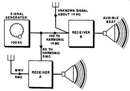
Fig. 10-9. Set-up for using the signal generator as a frequency standard.
WWV transmits with an extremely high degree of accuracy on frequencies of 2.5, 5, 10, 15, 20, 25, 30, and 35 mhz. Transmissions on 5, 10, 15, and 20 mhz may be received more readily due to the higher transmitting powers employed. In addition, standard audio frequencies of 440 hz and 600 hz are transmitted on all but the two higher frequencies in alternate 4-minute periods, with 1-minute pauses between, for time-signal announcements. Also, modulation by pulses spaced exactly 1 second apart may be heard.
Let us consider a practical example, illustrated by Fig. 10-9. We wish to measure the frequency of a station near 14 mhz, which is being received on receiver B. The output of the signal generator is connected to both receiver A and receiver B. Receiver A is tuned to WWV at 5 mhz. When the signal generator is adjusted to 100 khz, a beat note should be heard, as the 50th harmonic of the generator output heterodynes with the 5 mhz signal in receiver A. The signal generator is tuned for lower and lower beat-note pitch until zero beat, or very near it, is obtained. When the frequencies are very close together, a "pulsing" effect will be heard between them, indicating that they are within several cycles per second of each other. How close this relation can be maintained depends upon how stable the signal generator is, and how clean a signal it puts out on the higher harmonics. When the frequency of the generator has been carefully adjusted as close as possible to 100 khz, the harmonics in the 14 mhz region are found on receiver B, and the relative position of the unknown signal is determined accurately.
In some cases, the harmonics at the higher short-wave frequencies may be too weak and 200 khz, or 500 khz may have to be used for the fundamental. It will also be noticed that either the even or odd harmonics will be favored in some cases.
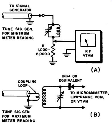
Fig. 10-10. Set-up for determining the resonant frequency of a tuned circuit.
10-10. Determining Resonant Frequency of a Tuned Circuit
Sometimes it is desirable to determine the resonant frequency of a coil and capacitor combination. One way to do this with a signal generator is illustrated in Fig. 10-10 (A). The coil and capacitor are connected in parallel and the combination is connected in series with a resistor (of 1,000 to 2,000 ohms). The whole combination is then connected across the output of a signal generator. A vacuum-tube voltmeter or a volt-ohm-milliammeter with a high-frequency probe is used to measure the r-f voltage across the resistor. When the signal generator is tuned through the resonant frequency, a marked change in the voltage across the resistor takes place. Ordinarily the voltage will dip, due to the rise in impedance of the tuned circuit to a high value at resonance. However, in some cases, the voltage may actually rise at resonance, because of poor regulation of the signal generator output voltage and possible capacitive effects between leads and parts of the circuit. In any event, the resonant frequency can be recognized as that at which the voltage across R changes suddenly, as the generator frequency is tuned through it. The meter may also be connected directly across the tuned circuit.
In this case the voltage indicated by the meter will be a maximum when the generator is tuned to the frequency of the parallel circuit.
A second method is shown in Fig. 10-10 (B). Here a small coupling loop consisting of several turns of insulated wire is connected to the output of the signal generator. A microammeter, a sensitive (20,000 ohms/volt) volt-ohm-milliammeter set to its lowest d-c voltage range, or a VTVM is connected through a crystal rectifier across the tuned circuit.
When the signal generator is tuned through the frequency of the circuit being checked, a noticeable peak in meter reading occurs. Peaks will also occur at harmonic frequencies of the generator; hence, the highest frequency peak should be utilized.
10-11. Using a Signal Generator as a Grid-Dip Meter
Without too much trouble, an a-m signal generator can be used as a grid-dip meter, which can then be used to check the resonant frequency of any tuned circuit within its range. In fact, with a grid-dip meter, a receiver or transmitter can be completely aligned without any power being applied.
The principle applied in the grid-dip meter is that, whenever the coil of an oscillator is loaded by the presence of a nearby circuit tuned to the same frequency, the grid current (and thus the self-bias across the grid resistor) drops to a relatively low value. Consequently, if the oscillator is brought into the presence of a tuned circuit and tuned through the resonant frequency of that circuit, the grid current of the oscillator dips quickly and returns to normal as the oscillator frequency passes through the tuned circuit frequency. The frequency of resonance of the tuned circuit is then determined by noting the point on the grid-dip oscillator dial at which the dip takes place.
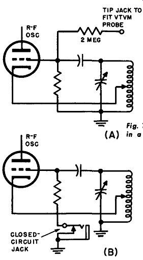
Fig. 10-11 Two methods of providing resonance indication in a signal generator
circuit, when the signal generator is to be used as a grid-dip meter.
Two things are necessary to convert a signal generator to a grid-dip meter: (1) some means of coupling its output to the circuits to be tested, and (2) some way of measuring grid current or d-c grid voltage.
The coupling can be provided by a loop of wire whose ends are connected to the ends of a lead plugged into the "high output" jack of the generator. If this coupling is not sufficient, a link around the generator coil (loosely coupled) can be connected to a lead with a loop of wire at the other end, which is placed near the circuit to be tested.
Figure 10-11 shows two ways of obtaining an indication of the grid dip. In (A) a vacuum-tube voltmeter is connected through a high resistance to the grid of the oscillator. In (B) the low side of the grid resistor is disconnected from ground and a dosed-circuit jack inserted.
In (A) a d-c VTVM is used, in (B), a microammeter with a range of about 0-500 µ.a is suitable.
The above modifications are appropriate for any of the lower priced signal generators designed for servicing use. However, it is not recommended that they be attempted with any precision laboratory types in which accurate output voltage indications are possible, as the accuracy of voltage and frequency may be affected.
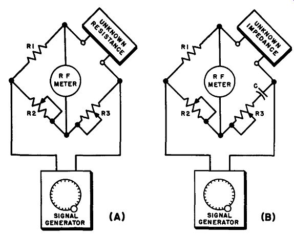
Fig. 10-12. (A) Wheatstone bridge connected to measure the r-f resistance
of a component. (B) Adapting the same principle to the impedance bridge, which
measures r-f impedance at the frequency of the generator.
10-12. Use of A-M Signal Generator in Impedance Bridge
An a-m signal generator can be used as the source of signal for operation of an impedance bridge. Its wide range of frequency and control of amplitude by attenuators makes it especially suitable for this purpose. The only special requirement is that, because the output voltage of the generator is relatively low, a sensitive indicator is required for determination of the null.
Figure 10-12 shows the circuits of a Wheatstone bridge and an impedance bridge which operates on the same principle. The wheatstone bridge (A) in its basic form, uses a d-c source of voltage and a d-c indicating instrument to indicate d-c resistance. By changing the voltage source to an a-m unmodulated signal generator, and the indicating instrument to one sensitive to r-f, we can make the bridge measure r-f resistance, as shown at (A). Of course, the ratio resistors R1 and R2, and the standard resistor R3 must be noninductive and be accurate for the frequency used. It is also preferable that they be shielded from each other.
The impedance bridge is the same as the resistance bridge except that the standard becomes an impedance instead of a pure resistance.
At (B), the bridge becomes an impedance bridge by the addition of the standard capacitor C; R3 is kept in the circuit to provide a sharper null by balancing out the resistance in the unknown impedance, but does not affect the impedance reading, which depends upon the reactance of C and the ratio of R1 and R21
• It has been stated that the indicator must be a sensitive one, due to the low output voltage of the generator. A crystal rectifier and micro ammeter will usually be found suitable. For even better sensitivity, and other advantages in some cases, a radio receiver, tuning to the frequency used in testing, can be employed as the indicator. If the receiver has an S-meter, an excellent indication is given. If not, it is recommended that the signal generator signal be modulated. Then the null point can be determined by listening to the receiver output.
IV. GENERAL APPLICATIONS OF SWEEP GENERATORS
10-13. R-F and I-F Transformer Response
The frequency response of individual components, as well as complete receivers and receiver sections, can be checked with a sweep generator. For example, consider such components as r-f and i-f transformers.
Some kind of response curve could be obtained by feeding a sweep signal into the primary winding and connecting the oscilloscope to the secondary winding (through a detector). However, with such a direct connection, it is difficult to match the conditions of load and stray capacitance actually encountered in a circuit. For this reason, a standard circuit is usually used which is so arranged that the transformers can be connected into this circuit quite easily. The whole circuit is then checked with the sweep generator in the same way as explained in Section 9.
Manufacturers of r-f and i-f transformers often specify their performance by stating what they will do in a given standard circuit.
--------------
1. The basic principles of bridge operation are quite standard, and the reader is referred to any good basic book on electricity for them.
--------------
10-14. Checking Filter Response
Since the use of tv receivers has become general, the problems of interference to tv reception have been given considerable attention. This has resulted in the wide use of high-pass filters on tv receivers, and low-pass filters on radio transmitters. By the use of a sweep analysis set-up as described for the tv receiver in Section 9, the characteristic of such a filter can be observed on the oscilloscope screen.
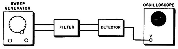
Fig. 10-13. Set-up for checking the response characteristic of a filter with
a sweep generator and oscilloscope.
The arrangement is shown in Fig. 10-13. The sweep generator output is fed to the input of the filter in the same way it would be coupled to a receiver. Most of the receiver-type high-pass filters are designed for 300-ohm input, so the same termination as for a 300-ohm receiver input is appropriate. The output of the filter is then connected to a detector whose input impedance is also 300 ohms. If the detector is a high- impedance device, it is necessary to add a 300-ohm termination on the output of the detector. With an unbalanced detector (one side grounded), two 150-ohm composition resistors may be used for termination, and the detector probe is then connected across one of the two terminating resistors. The output of the detector is connected to the vertical circuit of the oscilloscope. A marker generator must be used to check the cut-off frequency. This may usually be coupled by simply holding the hot lead near the filter itself. A typical high-pass filter characteristic, showing the marker pip, is shown in Fig. 10-14.
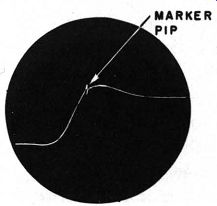
Fig. 10-14. Typical high-pass filter response as swept out on an oscilloscope,
with a marker of the cut-off frequency.
10-15. Indicating Standing Waves
With a suitable associated circuit, a sweep generator can be used to indicate, by a pattern on an oscilloscope screen, whether or not a trans mission line is properly terminated, by showing whether or not there are standing waves present. This is very useful in checking tv and f-m receiving antennas, and in checking certain types of transmitting antennas within the limitations which will be explained.
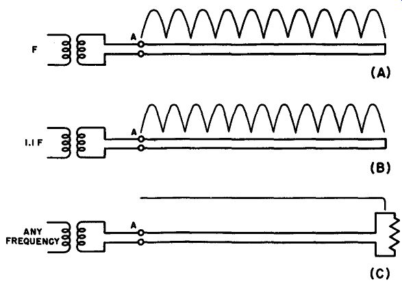
Fig. 10-15. Diagrams showing how the standing-wave distribution along an unmatched
line changes as frequency changes. (A) Standing waves along a line 10 half-wavelengths
long. (B) Standing waves along the some line when the frequency has been increased
to make the line 11 half-wavelengths long. (C) Constant voltage without standing
waves on a line which is terminated in its own characteristic impedance.
It has been previously explained how standing waves come to exist on a transmission line which is not terminated in its own characteristic impedance (Section 7-4). In Fig. 10-15 (A) is shown the representation of a transmission line into which is coupled r-f energy at frequency f.
The line is assumed not to be matched at its termination, so standing waves result, as shown in the figure. In the case assumed, the mismatch is such as to produce an even 10 cycles of voltage waves along the line, so there is zero voltage (or a minimum) at point a. Now suppose the frequency of the signal coupled into the line is increased to 1.1f. Since the line is still the same length, and the voltage peaks are still one-half wavelength apart, there are now 11 cycles of standing-wave variation instead of 10. Now if the frequency had been slowly increased from f to 1.1f, the voltage at point a would have varied gradually from zero (or some minimum value) up to a maximum and down to zero (or minimum) again. If the frequency were varied from f to 1.2f, this variation of voltage at a would take place twice. Therefore, variation of frequency input at a causes variations in voltage at point a, if the line is not matched.
Now suppose the line is matched. The standing waves then disappear, and there is a constant voltage all along the line, as shown at (C). There is thus a constant voltage at point a, and this voltage remains the same regardless of variations in the frequency of the r-f energy coupled into the line.
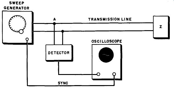
Fig. 10-16. Set-up for checking standing waves on a line with a sweep generator
and on oscilloscope.
With these ideas in mind, consider the set-up for checking standing waves as illustrated in Fig. 10-16. A sweep signal is coupled into the line from a sweep generator. The voltage at point a (input) of the line is rectified by a detector connected at that point. (Note: It is usually necessary to insert an impedance matching network at point a to match the output of the signal generator to the input of the transmission line.
Also, if the detector is a high-impedance device that is not balanced, two equal-value composition resistors (150 ohms each for a 300-ohm line) are connected in series across the line and their junction is grounded.
The detector is then connected across one of these resistors.) The output of the detector is connected to the oscilloscope vertical deflection circuit, and the oscilloscope horizontal circuit is synchronized to the sweep generator. Because of the change of r-f voltage at point a, the sweep line on the oscilloscope will be wavy. The number of waves across the screen will he the number of standing wave cycles passed through during the sweep frequency width. Adjustments in the terminating impedance Z can then be made until the wavy line on the oscilloscope screen straightens out and becomes a straight line. The straight-line trace indicates that the standing waves have disappeared and the transmission line is matched.
Certain limiting factors in this method should be noted. First, its use is limited if the terminating impedance of the line has a sharp frequency characteristic, such as would be exhibited by many transmitting antennas. With such a device, the transmission line would be matched only at or very near the frequency for which it is designed, and swinging the input frequency away from this frequency would indicate mis match even though there is none at the operating frequency. Thus, before the above method can be useful, the terminating impedance must be determined to have an impedance which is constant over the sweep range.
The second limiting factor is that the sweep range necessary to show at least one cycle of standing waves on the oscilloscope screen depends upon the length of line used in the test. If we think of a piece of line only one-half wavelength long, which has only one-half cycle of a standing wave along it, we will realize that before the input voltage will go through a complete cycle, we must change frequency to twice the original value. Now if we increase the line length to one full wave length, there will be two half cycles of standing waves, and an entire variation of standing waves will be completed when the frequency is increased to 3/2 its original value and so on for further increases. Considering these facts, we will realize that the ratio of change in frequency to produce at least one cycle of standing-wave voltage change at the input is:
f2 n + I fl n
where f_1 is the lowest frequency of the sweep f_2 is the upper edge of the frequency sweep n is the number half-wavelengths of standing waves along the line at the lowest frequency.
This formula is derived assuming a starting frequency at the lowest sweep value, rather than at the center, but is so close to the latter condition for a long enough line for the test that the difference is negligible.
Consider now the case of Fig. 10-15. If the starting frequency is 50 mhz at (A), then the frequency at (B) is 55 mhz. Therefore, to produce at least one standing wave variation cycle (at the input) on the oscilloscope, the generator frequency must sweep through at least 5 mhz. If the terminating impedance of the line is an antenna whose impedance changes radically at 51 mhz and 49 mhz, standing waves will be indicated even though the line is matched at 50 mhz, and the test is not of much use. On the other hand, if the termination is a broad-band tv receiving antenna, its impedance should not vary much over a wide range, and the test is satisfactory.
The length of line necessary for 10 half cycles of standing waves at 50 mhz would be nearly 100 ft. If the line length or the frequency is doubled, the frequency change necessary to produce a cycle of variation is cut in half, or would be only 2.5 mhz in this case.
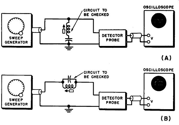
Fig. 10-17. Method used to check resonant frequency on a tuned circuit.
10-16. Measurement of Resonant Frequency
A sweep generator may be used to check the resonant frequency of a tuned circuit in the set-up shown in Fig. 10-17. A properly terminated sweep generator is used whose output is reasonably uniform over the approximate frequency range of the tuned circuit to be checked. In part (A) of the figure, the coil and capacitor are wired in series and this combination is shunted across the output of the sweep generator. An oscilloscope is connected through a detector probe to this circuit as shown. Under these conditions a marked dip occurs in the response curve at the resonant frequency of the L-C circuit. The coil and capacitor may also be wired in parallel and this combination connected in series with the hot lead as shown in part (B) of the figure. With this arrangement, it might be thought that a reduction in response will also occur here due to the high impedance of the parallel circuit at resonance. However, in practice, a marked rise (peak) may occur at the resonant frequency of the circuit. This is probably due to the marked reduction in sweep generator loading at resonance, which causes its output to rise.
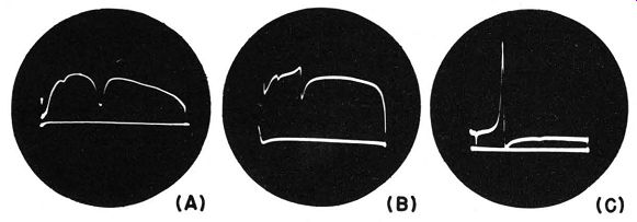
Fig. 10-18. Response curves produced with the set-up shown in the previous
figure.
Figure 10-18 shows the response curves obtained with the set-ups of Fig. 10-17. These response curves represent sweeps from 0 mhz (at the extreme left) to about 10 or 15 mhz (at the extreme right). In all cases, sweep generator blanking is used to produce the straight base line below the response curve. For Fig. 10-18 (A), the coil and capacitor are wired in series and this combination is shunted across the output of the sweep generator (as shown in Fig. 10-17 A). A marked dip (reduction in response) occurs at a frequency that was later marked to be about 4.5 mhz. For Fig. 10-18 (B), the coil and capacitor are wired in parallel and this combination is inserted in series with the hot lead of the sweep generator (as shown in Fig. 10-17B). A slight peak in the response curve occurs at the resonant frequency (marked later with a marker generator). This peak is followed immediately by a dip that occurs at a frequency slightly above the resonant frequency of the circuit. When this same arrangement was tried with another sweep generator, the response curve shown at Fig. 10-18 (C) was produced. Here the peak, which occurred at the resonant frequency of the L-C circuit, was very marked.
This peak was followed immediately by a dip at a frequency slightly above resonance.
It was found with the above set-up that the resonant frequency measured with the coil and capacitor connected together in series (as in Fig. 10-17A) was somewhat more accurate than when the parallel hook up (as in Fig. 10-17B) was used. In the latter case, shunting capacitance effects lowered the resonant frequency slightly.