|
|
__5 Interface Problems in Systems
If properly designed balanced interfaces were used throughout an audio system, it would theoretically be noise-free. Until about 1970, equipment designs allowed real-world system to come very close to this ideal. But since then, balanced interfaces have fallen victim to two major design problems-and both can properly be blamed on equipment manufacturers. Even careful examination of manufacturers' specifications and data sheets will not reveal either problem-the devil is in the details. These problems are effectively concealed because the marketing departments of most manufacturers have succeeded in dumbing down their so-called specifications over the same time period.
First is degraded noise rejection, which appeared when solid-state differential amplifiers started replacing input transformers. Second is the pin 1 problem that appeared in large numbers when PC boards and plastic connectors replaced their metal counterparts. Both problems can be avoided through proper design, of course, but in this author's opinion, part of the problem is that the number of analog design engineers who truly under stand the underlying issues is dwindling and engineering schools are steering most students into the digital future where analog issues are largely neglected.
Other less serious problems with balanced interfaces are caused by balanced cable construction and choices of cable shield connections.
On the other hand, unbalanced interfaces have an intrinsic problem that effectively limits their use to only the most electrically benign environments. Of course, even this problem can be solved by adding external ground-isolation devices, but the best advice is to avoid them whenever possible in professional systems!
__5.1 Degraded Common-Mode Rejection
Balanced interfaces have traditionally been the hallmark of professional sound equipment. In theory, systems comprised of such equipment are completely noise-free.
However, an often overlooked fact is that the common-mode rejection of a complete signal interface does not depend solely on the receiver, but on how the receiver interacts with the driver and the line performing as a subsystem.
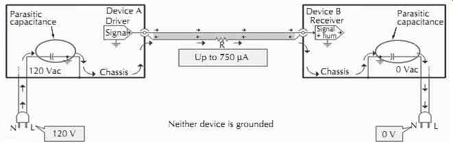
Figure 25. For ungrounded equipment, interconnect cables complete a capacitive
loop.
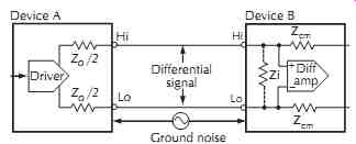
Figure 26. Simplified balanced interface.
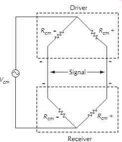
Figure 27. The balanced interface is a Wheatstone bridge.
In the basic balanced interface of FIG. 26, the output impedances of the driver Zo/2 and the input impedances of the receiver Zcm effectively form the Wheatstone bridge shown in FIG. 27. If the bridge is not balanced or nulled, a portion of the ground noise Vcm will be converted to a differential signal on the line.
This nulling of the common-mode voltage is critically dependent on the ratio matching of the pairs of driver/receiver common-mode impedances Rcm in the - and + circuit branches. The balancing or nulling is unaffected by impedance across the two lines, such as the signal input impedance Zi in FIG. 28 or the signal output impedance of the driver. It is the common-mode impedances that matter!
The bridge is most sensitive to small fractional impedance changes in one of its arms when all arms have the same impedance.
It is least sensitive when the upper and lower arms have widely differing impedances--e.g., when upper arms are very low and lower arms are very high, or vice versa. Therefore, we can minimize the sensitivity of a balanced system (bridge) to impedance imbalances by making common-mode impedances very low at one end of the line and very high at the other. This condition is consistent with the requirements for voltage matching discussed in Section 3.2.
Most active line receivers, including the basic differential amplifier of FIG. 28, have common-mode input impedances in the 5 k-ohm to 50 k-ohm range, which is inadequate to maintain high CMRR with real-world sources. With common-mode input impedances of 5k-ohm, a source imbalance of only 1-ohm , which could arise from normal contact and wire resistance variations, can degrade CMRR by 50 dB. Under the same conditions, the CMRR of a good input transformer would be unaffected because of its 50 M-ohm common-mode input impedances. FIG. 29 shows computed CMRR versus source imbalance for different receiver common-mode input impedances. Thermal noise and other limitations place a practical limit of about 130 dB on most actual CMRR measurements.
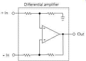
Figure 28. Basic differential amplifier.
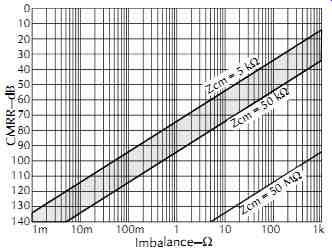
Figure 29. Noise rejection versus source impedance/imbalance.
How much imbalance is there in real-world signal sources? Internal resistors and capacitors determine the output impedance of a driver. In typical equipment, Zo/2 may range from 25 to 300-ohm. Since the resistors are commonly ±5% tolerance and the coupling capacitors are ±20% at best, impedance imbalances up to about 20-ohm should be routinely expected. This defines a real-world source. In a previous paper, this author has examined balanced audio interfaces in some detail, including performance comparisons of various receiver types. It was concluded that, regardless of their circuit topology, popular active receivers can have very poor CMRR when driven from such real-world sources. The poor performance of these receivers is a direct result of their low common-mode input impedances. If common-mode input impedances are raised to about 50 M-ohm , 94 dB of ground noise rejection is attained from a completely unbalanced 1 k: source, which is typical of consumer outputs. When common-mode input impedances are sufficiently high, an input can be considered truly universal, suitable for any source- balanced or unbalanced. A receiver using either a good input transformer or the InGenius integrated circuit will routinely achieve 90-100 dB of CMRR and remain unaffected by typical real-world output imbalances.
The theory underlying balanced interfaces is widely misunderstood by audio equipment designers. Pervasive use of the simple differential amplifier as a balanced line receiver is evidence of this. And, as if this weren't bad enough, some have attempted to improve it.
Measuring input X and Y input impedances of the simple differential amplifier individually leads some designers to alter its equal resistor values. However, as shown in FIG. 30, if the impedances are properly measured simultaneously, it becomes clear that nothing s wrong. The fix grossly unbalances the common-mode impedances, which destroys the interface CMRR for any real-world source. This and other misguided improvements completely ignore the importance of common-mode input impedances.
The same misconceptions have also led to some CMRR tests whose results give little or no indication of how the tested device will actually behave in a real-world system. Apparently, large numbers of designers test the CMRR of receivers with the inputs either shorted to each other or driven by a laboratory precision signal source. The test result is both unrealistic and misleading. Inputs rated at 80 dB of CMRR could easily deliver as little as 20 dB or 30 dB when used in a real system. Regarding their previous test, the IEC had recognized that test is not an adequate assurance of the performance of certain electronically balanced amplifier input circuits. The old method simply didn't account for the fact that source impedances are rarely perfectly balanced. To correct this, this author was instrumental in revising IEC Standard: 60268-3 Sound System Equipment - Part 3: Amplifiers.
The new method, as shown in FIG. 31, uses typical ±10-ohm source impedance imbalances and clearly reveals the superiority of input transformers and some new active input stages that imitate them. The new standard was published August 30, 2000. The Audio Precision APx520 and APx525, introduced in 2008, are the first audio instruments to offer the new CMRR test.
__5.2 The Pin 1 Problem
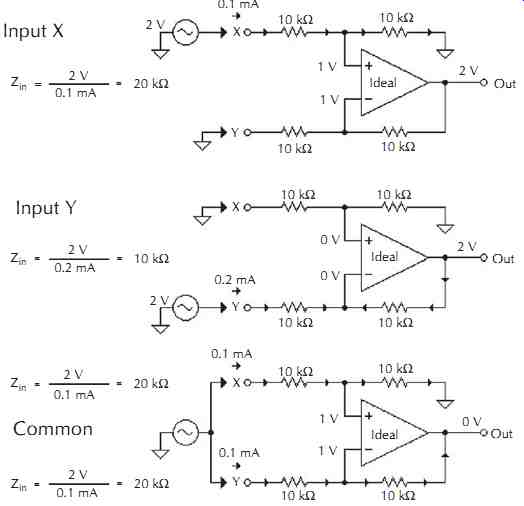
Figure 30. Common-mode impedances apply to a voltage applied to both inputs.
In his now famous paper in the 1995 AES Journal, Neil Muncy says:
This paper specifically addresses the problem of noise coupling into balanced line-level signal interfaces used in many professional applications, due to the unappreciated consequences of a popular and widespread audio equipment design practice which is virtually without precedent in any other field of electronic systems.
Common impedance coupling occurs whenever two currents flow in a shared or common impedance. A noise coupling problem is created when one of the currents is ground noise and the other is signal. The common impedance is usually a wire or circuit board trace having a very low impedance, usually well under an ohm. Unfortunately, common impedance coupling has been designed into audio equipment from many manufacturers. The noise current enters the equipment via a terminal, at a device input or output, to which the cable shield is connected via a mating connector. For XLR connectors, it's pin 1 (hence the name); for ¼ inch connectors, it's the sleeve; and for RCA/IHF connectors, it's the shell.
To the user, symptoms are indistinguishable from many other noise coupling problems such as poor CMRR. To quote Neil again, Balancing is thus acquiring a tarnished reputation, which it does not deserve. This is indeed a curious situation. Balanced line-level interconnections are supposed to ensure noise-free system performance, but often they do not.
In balanced interconnections, it occurs at line inputs and outputs where interconnecting cables routinely have their shields grounded at both ends. Of course, grounding at both ends is required for unbalanced interfaces.
Fig.32 illustrates several examples of common impedance coupling. When noise currents flow in signal reference wiring or circuit board traces, tiny voltage drops are created. These voltages can couple into the signal path, often into very high gain circuitry, producing hum or other noise at the output. In the first two devices, pin 1 current is allowed to flow in internal signal reference wiring. In the second and third devices, power line noise current (coupled through the parasitic capacitances in the power transformer) is also allowed to flow in signal reference wiring to reach the chassis/safety ground. This so-called sensitive equipment will produce additional noise independent of the pin 1 problem. For the second device, even disconnecting its safety ground (not recommended) won't stop current flow through it between input and output pin 1 shield connections.
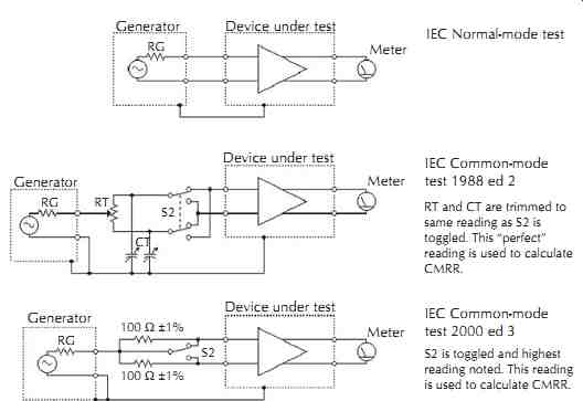
Figure 31. Old and new IEC tests for CMRR compared.
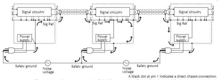
Figure 32. How poor routing of shield currents produces the pin 1 problem.
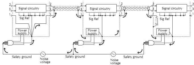
Figure 33. Equipment with proper internal grounding.
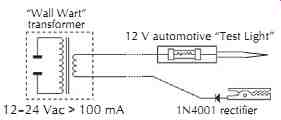
Figure 34. The Hummer II. Jensen Transformers, Inc.
FIG. 33 shows three devices whose design does not allow shield current to flow in signal reference conductors. The first uses a star connection of input pin 1, output pin 1, power cord safety ground, and power supply common. This technique is the most effective prevention. Noise currents still flow, but not through internal signal reference conductors. Before there were printed circuit boards, a metal chassis served as a very low-impedance connection (effectively a ground plane) connecting all pins 1 to each other and to safety ground. Pin 1 problems were virtually unknown in those vintage designs. Modern printed circuit board-mounted connectors demand that proper attention be paid to the routes taken by ground noise currents. Of course, this same kind of problem can and does exist with RCA connectors in unbalanced consumer equipment, too.
Fortunately, tests to reveal such common impedance coupling problems are not complex. Comprehensive tests using lab equipment covering a wide frequency range have been described by Cal Perkins and simple tests using an inexpensively built tester called the hummer have been described by John Windt. Jensen Transformers, Inc. variant of the Hummer is shown in FIG. 34. It passes a rectified ac current of 60-80 mA through the potentially troublesome shield connections in the device under test to determine if they cause the coupling.
The glow of the automotive test lamp shows that a good connection has been made and that test current is indeed flowing. The procedure:
1. Disconnect all input and output cables, except the output to be monitored, as well as any chassis connections (due to rack mounting, for example) from the device under test.
2. Power up the device.
3. Meter and, if possible, listen to the device output.
Hopefully, the output will simply be random noise.
Try various settings of operator controls to familiarize yourself with the noise characteristics of the device under test without the hummer connected.
4. Connect the hummer clip lead to the device chassis and touch the probe tip to pin 1 of each input or output connector. If the device is properly designed, there will be no output hum or change in the noise floor.
5. Test other potentially troublesome paths, such as from an input pin 1 to an output pin 1 or from the safety ground pin of the power cord to the chassis (a three-to-two-prong ac adapter is handy to make this connection).
Note: Pin 1 might not be connected directly to ground in some equipment-hopefully, this will be at inputs only! In this case, the hummer's lamp may not glow--this is OK.
__5.3 Balanced Cable Issues
At audio frequencies, even up to about 1 MHz, cable shields should be grounded at one end only, where the signal is ground referenced. At higher frequencies, where typical system cables become a small fraction of a wavelength, it's necessary to ground it at more than one point to keep it at ground potential and guard against RF interference. Based on my own work, there are two additional reasons that there should always be a shield ground at the driver end of the cable, whether the receiver end is grounded or not, see FIGs. 35 and 36. The first reason involves the cable capacitances between each signal conductor and shield, which are mismatched by 4% in typical cable. If the shield is grounded at the receiver end, these capacitances and driver common-mode output impedances, often mismatched by 5% or more, form a pair of low-pass filters for common-mode noise. The mismatch in the filters converts a portion of common-mode noise to differential signal. If the shield is connected only at the driver, this mechanism does not exist. The second reason involves the same capacitances working in concert with signal asymmetry. If signals were perfectly symmetrical and capacitances perfectly matched, the capacitively coupled signal current in the shield would be zero through cancellation. Imperfect symmetry and/or capacitances will cause signal current in the shield. This current should be returned directly to the driver from which it came. If the shield is grounded at the receiver, all or part of this current will return via an undefined path that can induce crosstalk, distortion, or oscillation.
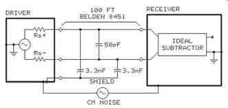
Figure 35. Shield grounded only at driver.
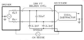
Figure 36. Shield grounded only at receiver.
With cables, too, there is a conflict between the star and mesh grounding methods as discussed in Section 4.3. But this low-frequency versus high-frequency conflict can be substantially resolved with a hybrid approach involving grounding the receive end of cables through an appropriate capacitance (shown in the third device of FIG. 33). Capacitor values in the range of 10 nF to 100 nF are most appropriate for the purpose.
Such capacitance has been integrated into the Neutrik EMC series connectors. The merits of this scheme were the subject of several years of debate in the Audio Engineering Society Standards Committee working group that developed AES48.
As discussed in Section 2.5, twisting essentially places each conductor at the same average distance from the source of a magnetic field and greatly reduces differential pickup. Star quad cable reduces pickup even further, typically by about 40 dB. But the downside is that its capacitance is approximately double that of standard shielded twisted pair.
SCIN, or shield-current induced noise, may be one consequence of connecting a shield at both ends. Think of a shielded twisted pair as a transformer with the shield acting as primary and each inner conductor acting as a secondary winding, as shown in the cable model of FIG. 37. Current flow in the shield produces a magnetic field which then induces a voltage in each of the inner conductors. If these voltages are identical, and the interface is properly impedance balanced, only a common-mode voltage is produced that can be rejected by the line receiver. However, subtle variations in physical construction of the cable can produce unequal coupling in the two signal conductors. The difference voltage, since it appears as signal to the receiver, results in noise coupling. Test results on six commercial cable types appear in reference. In general, braided shields perform better than foil shields and drain wires.
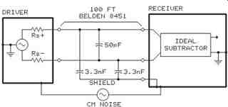
Figure 37. Shield of a shielded twisted pair cable is magnetically coupled
to inner conductors.
And, to make matters even worse, grounding the shield of balanced interconnect cables at both ends also excites the pin 1 problem if it exists. Although it might appear that there's little to recommend grounding at both ends, it is a widely accepted practice. As you can see, noise rejection in a real-world balanced interface can be degraded by a number of subtle problems and imperfections. But, as discussed in Section 6.4, it is virtually always superior to an unbalanced interface!
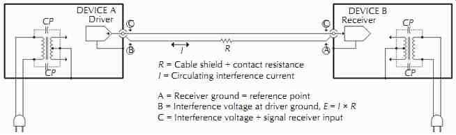
Figure 38. Common impedance coupling in an unbalanced audio, video, or data
interface.
__5.4 Coupling in Unbalanced Cables
The overwhelming majority of consumer as well as high-end audiophile equipment still uses an audio inter face system introduced over 60 years ago and intended to carry signals from chassis to chassis inside the earliest RCA TV receivers! The ubiquitous RCA cable and connector form an unbalanced interface that is extremely susceptible to common impedance noise coupling.
As shown in FIG. 38, noise current flow between the two device grounds or chassis is through the shield conductor of the cable. This causes a small but significant noise voltage to appear across the length of the cable. Because the interface is unbalanced, this noise voltage will be directly added to the signal at the receiver. In this case, the impedance of the shield conductor is responsible for the common impedance coupling. This coupling causes hum, buzz, and other noises in audio systems. It's also responsible for slow-moving hum bars in video interfaces and glitches, lock-ups, or crashes in unbalanced--e.g., RS-2 data interfaces.
Consider a 25 ft interconnect cable with foil shield and a #26 AWG drain wire. From standard wire tables or actual measurement, its shield resistance is found to be 1.0-ohm. If the 60 Hz leakage current is 300 µA, the hum voltage will be 300 µV. Since the consumer audio reference level is about -10 dBV or 300 mV, the 60 Hz hum will be only relative to the signal. For most systems, this is a very poor signal-to-noise ratio! For equipment with two-prong plugs, the 60 Hz harmonics and other high-frequency power-line noise (refer to FIG. 20) will be capacitively coupled and result in a harmonic-rich buzz.
Because the output impedance of device A and the input impedance of device B are in series with the inner conductor of the cable, its impedance has an insignificant effect on the coupling and is not represented here.
Common-impedance coupling can become extremely severe between two grounded devices, since the voltage drop in the safety ground wiring between the two devices is effectively parallel connected across the length of the cable shield. This generally results in a fundamental-rich hum that may actually be larger than the reference signal!
Coaxial cables, which include the vast majority of unbalanced audio cables, have an interesting and under appreciated quality regarding common-impedance coupling at high frequencies, FIG. 39. Any voltage appearing across the ends of the shield will divide itself between shield inductance Ls and resistance Rs according to frequency. At some frequency, the voltages across each will be equal (when reactance of Ls equals Rs). For typical cables, this frequency is in the 2 to 5 kHz range. At frequencies below this transition frequency, most of the ground noise will appear across Rs and be coupled into the audio signal as explained earlier. However, at frequencies above the transition frequency, most of the ground noise will appear across Ls. Since Ls is magnetically coupled to the inner conductor, a replica of the ground noise is induced over its length. This induced voltage is then subtracted from the signal on the inner conductor, reducing noise coupling into the signal. At frequencies ten times the transition frequency, there is virtually no noise coupling at all-common-impedance coupling has disappeared.
Therefore, common-impedance coupling in coaxial cables ceases to be a noise issue at frequencies over about 50 kHz. Remember this as we discuss claims made for power line filters that typically remove noise only above about 50 kHz.
Unbalanced interface cables, regardless of construction, are also susceptible to magnetically induced noise caused by nearby low-frequency ac magnetic fields.
Unlike balanced interconnections, such noise pickup is not nullified by the receiver.
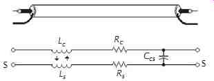
Figure 39. Magnetic coupling between shield and center conductor is 100%.
__5.5 Bandwidth and RF Interference
RF interference isn't hard to find-it's actually very difficult to avoid, especially in urban areas. It can be radiated through the air and/or be conducted through any cables connected to equipment. Common sources of radiated RF include AM, shortwave, FM, and TV broadcasts; ham, CB, remote control, wireless phone, cellular phone, and a myriad of commercial two-way radio and radar transmitters; and medical and industrial RF devices. Devices that create electrical sparks, including welders, brush-type motors, relays, and switches can be potent wideband radiators. Less obvious sources include arcing or corona discharge from power line insulators (common in seashore areas or under humid conditions) or malfunctioning fluorescent, HID, or neon lights. Of course, lightning, the ultimate spark, is a well-known radiator of momentary interference to virtually anything electronic.
Interference can also be conducted via any wire coming into the building. Because power and telephone lines also behave as huge outdoor antennas, they are often teeming with AM radio signals and other interference. But the most troublesome sources are often inside the building and the energy delivered through ac power wiring. The offending source may be in the same room as your system or, worse yet, it may actually be a part of your system! The most common offenders are inexpensive light dimmers, fluorescent lights, CRT displays, digital signal processors, or any device using a switching power supply.
Although cable shielding is a first line of defense against RF interference, its effectiveness depends critically on the shield connection at each piece of equipment. Because substantial inductance is added to this connection by traditional XLR connectors and grounding pigtails, the shield becomes useless at high radio frequencies. Common-mode RF interference simply appears on all the input leads.34 Because the wire limitations discussed in Section 2.4 apply to grounding systems, contrary to widespread belief, grounding is not an effective way to deal with RF interference. To quote Neil Muncy:
Costly technical grounding schemes involving various and often bizarre combinations of massive copper conductors, earth electrodes, and other arcane hardware are installed. When these schemes fail to provide expected results, their proponents are usually at a loss to explain why.
The wider you open the window, the more dirt flies in. One simple, but often overlooked, method of minimizing noise in a system is to limit the system band width to that required by the signal.
In an ideal world, every signal-processing device in a system would contain a filter at each input and output connector to appropriately limit bandwidth and prevent out-of-band energy from ever reaching active circuitry. This RF energy becomes an audio noise problem because the RF is demodulated or detected by active circuitry in various ways, acting like a radio receiver that adds its output to the audio signal. Symptoms can range from actual reception of radio signals or a 59.94 Hz buzz from TV signals or various tones from cell phone signals to much subtler distortions, often described as a veiled or grainy audio quality.37 The filters necessary to prevent these problems vary widely in effectiveness and, in some equipment, may not be present at all. Sadly, the performance of most commercial equipment will degrade when such interference is coupled to its input.
__6 Solving Real-World System Problems
How much noise and interference are acceptable depends on what the system is and how it will be used.
Obviously, sound systems in a recording studio need to be much more immune to noise and interference than paging systems for construction sites.
__6.1 Noise Perspective
The decibel is widely used to express audio-related measurements. For power ratios,
For voltage or current ratios, because power is proportional to the square of voltage or current:
Most listeners describe 10 dB level decreases or increases as halving or doubling loudness, respectively, and 2 dB or 3 dB changes as just noticeable. Under laboratory conditions, well-trained listeners can usually identify level changes of 1 dB or less. The dynamic range of an electronic system is the ratio of its maximum undistorted signal output to its residual noise output or noise floor. Up to 120 dB of dynamic range may be required in high-end audiophile sound systems installed in typical homes.
__6.2 Troubleshooting
Under certain conditions, many systems will be accept ably noise-free in spite of poor grounding and inter facing techniques. People often get away with doing the wrong things! But, notwithstanding anecdotal evidence to the contrary, logic and physics will ultimately rule.
Troubleshooting noise problems can be a frustrating, time-consuming experience but the method described in Section 6.2.2 can relieve the pain. It requires no electronic instruments and is very simple to perform. Even the underlying theory is not difficult. The tests will reveal not only what the coupling mechanism is but also where it is.
__6.2.1 Observations, Clues, and Diagrams
A significant part of troubleshooting involves how you think about the problem. First, don't assume anything! For example, don't fall into the trap of thinking, just because you've done something a particular way many times before, it simply can't be the problem. Remember, even things that can't go wrong, do! Resist the temptation to engage in guesswork or use a shotgun approach.
If you change more than one thing at a time, you may never know what actually fixed the problem.
Second, ask questions and gather clues! If you have enough clues, many problems will reveal themselves before you start testing. Be sure to write everything down-imperfect recall can waste a lot of time! Troubleshooting guru Bob Pease suggests these basic questions:
1. Did it ever work right?
2. What are the symptoms that tell you it's not working right?
3. When did it start working badly or stop working?
4. What other symptoms showed up just before, just after, or at the same time as the failure?
Operation of the equipment controls, and some elementary logic, can provide very valuable clues. For example, if a noise is unaffected by the setting of a gain control or selector, logic dictates that it must be entering the signal path after that control. If the noise can be eliminated by turning the gain down or selecting another input, it must be entering the signal path before that control.
Third, sketch a block diagram of the system.
FIG. 40 is an example diagram of a simple home theater system. Show all interconnecting cables and indicate approximate length. Mark any balanced inputs or outputs. Generally, stereo pairs can be indicated with a single line. Note any device that is grounded via a three-prong ac plug. Note any other ground connections such as equipment racks, cable TV connections, etc.
__6.2.2 The Ground Dummy Procedure
An easily constructed adapter or ground dummy is the key element in this procedure. By temporarily placing the dummy at strategic locations in the interfaces, precise information about the nature and location of the problem is revealed. The tests can specifically identify:
1. Common-impedance coupling in unbalanced cables.
2. Shield current-induced coupling in balanced cables.
3. Magnetic or electrostatic pickup of nearby magnetic or electrostatic fields.
4. Common-impedance coupling (the pin 1 problem) inside defective devices.
5. Inadequate CMRR of the balanced input.
The ground dummy can be made from standard connector wired as shown in FIGs. 41 and 42.
Since a dummy does not pass signal, mark it clearly to help prevent it, being accidentally left in a system.
Each signal interface is tested in four steps. As a general rule, always start at the inputs to the power amplifiers and work backward toward the signal sources. Be very careful when performing the tests not to damage loudspeakers or ears! The surest way to avoid possible damage is to turn off the power amplifier(s) before reconfiguring cables for each test step.
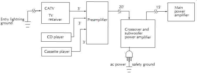
Figure 40. Block diagram of example system.
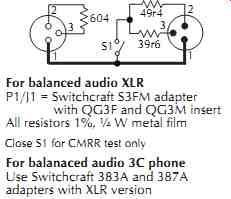
Figure 41. Balanced ground dummy.
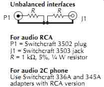
Figure 42. Unbalanced ground dummy.
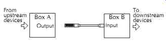
__6.2.2.1 For Unbalanced Interfaces
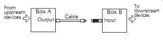 STEP 1: Unplug the cable from the input of Box B and plug in only the dummy
as shown below.
STEP 1: Unplug the cable from the input of Box B and plug in only the dummy
as shown below.
Output quiet?
No-The problem is either in Box B or farther downstream.
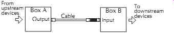
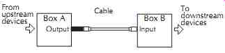
STEP 2: Leaving the dummy in place at the input of Box B, plug the cable into
the dummy as shown below.
STEP 3: Remove the dummy and plug the cable directly into the input of Box
B. Unplug the other end of the cable from the output of Box A and plug it into
the dummy as shown below. Do not plug the dummy into Box A or let it touch
anything conductive.
Output quiet?
No-Noise is being induced in the cable itself.
Reroute the cable to avoid interfering fields (see Section 4.2 or 4.4).
Yes-Go to next step.
STEP 4: Leaving the dummy in place on the cable, plug the dummy into the output
of Box A as shown below.
Output quiet?
No--The problem is common-impedance coupling (see Section 4.4). Install a ground isolator at the input of Box B.
Yes--The noise is coming from (or through) the output of Box A. Perform the same test sequence on the cable(s) connecting Box A to upstream devices.
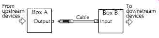
__6.2.2.2 For Balanced Interfaces
STEP 1: Unplug the cable from the input of Box B and plug in only the dummy
(switch open or NORM) as shown below.
Output quiet? No-The problem is either in Box B or farther downstream.
Yes--Go to next step.
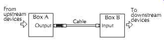
STEP 2: Leaving the dummy in place at the input of Box B, plug the cable into
the dummy (switch open or NORM) as shown below.
Output quiet?
No--Box B has a Pin 1 problem (see hummer test, Section 4.2, to confirm this).
Yes--Go to next step.
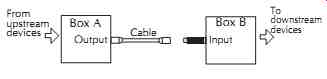
STEP 3: Remove the dummy and plug the cable directly into the input of Box
B. Unplug the other end of the cable from the output of Box A and plug it into
the dummy (switch open or NORM) as shown below. Do not plug the dummy into
Box A or let it touch anything conductive.
Output quiet?
No--Noise is being induced in the cable itself by an electric or magnetic field. Check the cable for an open shield connection, reroute the cable to avoid the interfering field, or replace the cable with a starquad type (see Sections 2.5 and 4.3).
Yes--Go to next step.
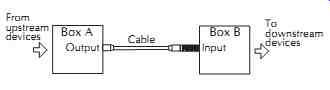
STEP 4: Leaving the dummy in place on the cable, plug the dummy (switch open
or NORM) into the output of Box A as shown below.
Output quiet?
No--The problem is shield-current-induced noise. Replace the cable with a different type (without a drain wire) or take steps to reduce current in the shield.
Yes--Go to next step.

STEP 5: Leave the dummy and cable as for step 4, but move the dummy switch
to the CMRR (closed) position.
Output quiet?
No--The problem is likely inadequate common-mode rejection of the input stage of Box B. This test is based on the IEC common mode rejection test but uses the actual common-mode voltage present in the system.
The nominal 10-ohm imbalance may not simulate the actual imbalance at the output of Box A, but the test will reveal input stages whose CMRR is sensitive to source imbalances. Most often, adding a transformer-based ground isolator at the input of Box B will cure the problem.
Yes--The noise must be coming from (or through) the output of Box A. Perform the same test sequence on the cable(s) connecting Box A to upstream devices.